This post is as applied as it gets for this blog. We will see how to manipulate multi-dimensional arrays as clean and efficient as possible. Being able to do so is an essential tool for any machine learning practitioner these days, much of what is done in python nowadays would not be possible without libraries such as NumPy, PyTorch and TensorFlow which handle heavy workloads in the background. This is especially true if you are working in computer vision. Images are represented as multi-dimensional arrays, and we frequently need to pre- and post-process them in an efficient manner in the ML-pipeline. In what follows, we will see some of the tools necessary for these tasks.

NumPy Basics

Before we can get into the details of vectorization and broadcasting we need to understand the basics of NumPy, especially its np.ndarray class. The power of NumPy lies in its ability to pass on python instructions to much more efficient C implementations, the same applies to mapping data structures to memory. Hence when using NumPy data structures we should only manipulate them with NumPy methods whenever possible.

For all of the following code snippets we will assume that numpy as imported as np.

import numpy as np

The np.ndarray Data Structure

At its core the np.ndarray is simply an array, similar to a list in python. However while in python you can have objects of different types in a list, the ndarray is homogeneous. It allows only objects of the same type to be present. Most frequently we will encounter the following types:

• np.int64: Also called long in other programming languages, a 64-bit signed integer. The default type for integer typed data.
• np.int32: Also called int in other programming languages, a 32-bit signed integer.
• np.float64: Double precision float, the default floating point type.
• np.float32: Single precision float.
• Many others are supported: float16 to float128, or int8 to int64, uint8 to uint64 for unsigned integer, object, string and bool.

NumPy takes great care to allocate the required memory for its arrays as efficiently as possible, this is something we should keep in when manipulating them. When we transform python lists to a ndarray the data type and shape will be inferred automatically. In general a ndarray has the following attributes:

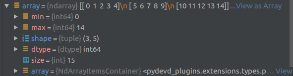
• min: minimum value in the array
• max: maximum value in the array
• shape: tuple containing the size of each dimension
• dtype: type of the objects in the array, see above for details
• size: number of elements in the array

Here is an example of the debug view of an array of shape (3,5) containing elements numbered from 0 to 14:

Generating Data

There are many ways to create a ndarray some of the most frequent ones are list here:

Python or PyTorch to ndarray

We can ask NumPy to transform a list, or a list of lists, to an ndarray using the np.array() method.

python_array = [[i*5+j for j in range(5)] for i in range(3)]
[[0, 1, 2, 3, 4], [5, 6, 7, 8, 9], [10, 11, 12, 13, 14]]
np.array(python_array)
array([[ 0,  1,  2,  3,  4],
       [ 5,  6,  7,  8,  9],
       [10, 11, 12, 13, 14]])

If you are using PyTorch, then there is an efficient way to transform tensors to ndarray objects using tensor.numpy(). This will not copy the data but instead give you direct access to the same memory space where the tensor is allocated. Hence if you change the NumPy object, the PyTorch object will be changed as well.

import torch
torch_array = torch.arange(15).reshape(3,5)
tensor([[ 0,  1,  2,  3,  4],
        [ 5,  6,  7,  8,  9],
        [10, 11, 12, 13, 14]])
torch_array.numpy()
array([[ 0,  1,  2,  3,  4],
       [ 5,  6,  7,  8,  9],
       [10, 11, 12, 13, 14]])

Deterministically Filled Arrays

We can create an array filled by ones or zeros using np.ones(shape) and np.zeros(shape). There is also the option to create an array filled with ones or zeros in the shape of another array, using np.ones_like(array) or np.zeros_like(array).

We can use np.arange(size).reshape(shape) to count from 0 to size-1 and transform it into the desired size.

size, shape = 15, (3, 5)
np.arange(size).reshape(shape)
array([[ 0,  1,  2,  3,  4],
       [ 5,  6,  7,  8,  9],
       [10, 11, 12, 13, 14]])
ones = np.ones(shape)
array([[1., 1., 1., 1., 1.],
       [1., 1., 1., 1., 1.],
       [1., 1., 1., 1., 1.]])
np.zeros_like(ones)
array([[0., 0., 0., 0., 0.],
       [0., 0., 0., 0., 0.],
       [0., 0., 0., 0., 0.]]

Randomly Filled Arrays

Arrays filled with random numbers are also possible, we can get random integers by calling np.random.randint(size, size=size).reshape(shape), which will draw integers from 0 to size-1. Or we can draw from a random normal distribution by using np.random.randn(*shape). Which is unfortunately an inconsistent interface compared to other methods which take a shape parameter.

size, shape = 15, (3, 5)
np.random.randint(size, size=size).reshape(shape)
array([[10, 11,  6,  3,  5],
       [13,  9,  1,  0,  7],
       [ 6,  8, 14, 14,  0]])
np.random.randn(*shape)
array([[-1.44118486,  0.92628989,  0.56191427, -0.78502917, -0.44458898],
       [ 0.07069683,  0.69491737,  1.43222532,  1.31024956, -1.44594812],
       [-0.43396544,  1.07042421, -1.33461508,  0.24587141, -0.40891315]])

Indexing and Views

To understand the manipulation of NumPy arrays, we will first need look at how to access parts of the array. Suppose we have an array which is a matrix, i.e. it has two dimensions (rows, columns). Then we can access elements either by using the standard python notation array[row][col] or use array[row, column]. The latter version is more concise and what we will use from now on.

For the rest of this section we will assume that we are manipulating this array

size, shape = 15, (3, 5)
array = np.arange(size).reshape(shape)
array([[ 0,  1,  2,  3,  4],
       [ 5,  6,  7,  8,  9],
       [10, 11, 12, 13, 14]])

Elements

Accessing and updating elements is simple, we can use the above introduced notation. Although the accesses element is still a NumPy type, it is not a pointer to the original memory space. Changing it will not update the matrix, we can update a matrix in the same way we access a single element:

elem = array[1, 2]
7
elem = 14
14
array([[ 0,  1,  2,  3,  4],
       [ 5,  6,  7,  8,  9],
       [10, 11, 12, 13, 14]])
array[1, 2] = 15
array([[ 0,  1,  2,  3,  4],
       [ 5,  6, 15,  8,  9],
       [10, 11, 12, 13, 14]])

Slicing or Views

If we continue with the same example above, we can extract the second row with the slicing operator array[1,:], where : means we want to select all the elements in that dimension. This will give us a “view” of the second row, which still points to the same memory space as the original array. Consequently if we manipulate it the original array will be updated to. Selecting a range of elements in an array works the same as in python lists. If you want to make a copy of an array, then you need to specify this explicitly using array.copy().

slice = array[1, :]
array([ 5,  6, 15,  8,  9])
slice[2] = 7
array([ 5,  6, 7,  8,  9])
array
array([[ 0,  1,  2,  3,  4],
       [ 5,  6,  7,  8,  9],
       [10, 11, 12, 13, 14]])
slice[1:3]
array([6, 7])

Fancy Indexing

If you would like to select non-contiguous parts of the array, this is also possible with fancy indexing. For example selecting the first and the last row can be done using array[[0, -1]], this will then return a copy of the selected rows. Hence updating it will not change the original array.

fancy_slice = array[[0,-1]]
array([[ 0,  1,  2,  3,  4],
       [10, 11, 12, 13, 14]])
fancy_slice[1,1] = 22
array([[ 0,  1,  2,  3,  4],
       [10, 22, 12, 13, 14]])
array
array([[ 0,  1,  2,  3,  4],
       [ 5,  6,  7,  8,  9],
       [10, 11, 12, 13, 14]])

Example: Transforming Class Labels to One-Hot Encoded Vectors

In a previous post on neural networks from scratch we loaded the MNIST data and the labels were simple numbers. However the training required one-hot encoded vectors. How can we efficiently create one from the other? By using the some of the functionalities we just saw above! Remember that a one hot encoded vector is one for the true class and zero everywhere else. So if we have an image which could be one of five classes, and has true label three, then we need to transform 3 to [0,0,0,1,0]. This method will do it for us in a few lines, supposing that the labels is an one dimensional array of shape (size) and the classes is the number of different classes which can appear:

def labels_to_one_hot(labels: np.ndarray, classes: int) -> np.ndarray:
    one_hot = np.zeros((labels.size, classes))
    one_hot[np.arange(labels.size), labels] = 1
    return one_hot

We dynamically select a row with arange which simply generates a sequence from 0 to labels.size -1, while labels will choose the column to be set to 1.

Vectorization

In short, vectorization is the process of replacing explicit loops with array expressions. In general, vectorization will speed up the calculation by one to three orders of magnitude. The speedup is achieved by delegating the work to a low-level language, such as C. A simple example is the calculation of an average of a large matrix. We will do this for the training data set of MNIST, which consists of 50’000 images with a resolution of 28x28. In the reshaped matrix version it has a shape of (50000, 784).

def matrix_average(matrix: np.ndarray) -> float:
    height, width = matrix.shape
    s = 0.0
    for i in range(height):
        for j in range(width):
            s += matrix[i, j]
    return s / (height*width)

x_train = get_mnist_training_images()

classic_average = matrix_average(x_train)
numpy_average = np.average(x_train)
classic_average, numpy_average
0.13044972207828445 0.13044983

Even just visually, NumPy has the clear advantage of being very clear and concise, the larger advantage is however in the speed:

from timeit import timeit
setup = 'from __main__ import classic_average, x_train; import numpy as np'
num = 10
t1 = timeit('classic_average(x_train)', setup=setup, number=num)
t2 = timeit('np.average(x_train)', setup=setup, number=num)
t1/num, t2/num, t1/t2
12.27550071660662 0.012771252996753902 961.1821737245917

When we run this simple example ten times, then on average the NumPy version is 961 times faster than the pure python implementation. The speedup is big because we are handling a large data set, but it will be noticeable for smaller tasks too. Maybe you think this task was too far fetched, and its rare that we want to calculate the average of that many images, then consider the next task.

Suppose we have a network which does semantic segmentation, that means it does classification for each pixel. If the input is an image of resolution (1280, 720) and we want to distinguish between 20 classes, then the output will be of shape (1280, 720, 20). The last dimension is then often the probability that class k is the true class, and we would like to find the maximum along that dimension to make a prediction. This process is called taking the arg max. We can again do this the naive way or using vectorized calculations:

def tensor_arg_max(tensor: np.ndarray) -> np.ndarray:
    width, height, classes = tensor.shape
    arg_max = np.zeros((width, height), dtype=np.int32)
    for i in range(width):
        for j in range(height):
            max_index, max_value = 0, 0
            for k in range(classes):
                if tensor[i, j, k] > max_value:
                    max_index, max_value = k, tensor[i, j, k]
            arg_max[i, j] = max_index
    return arg_max

shape = (1280, 720, 20)
random_network_output = np.random.random(size=np.prod(shape)).reshape(shape)
python_arg_max = tensor_arg_max(random_network_output)
numpy_arg_max = np.argmax(random_network_output, axis=2)

np.sum(np.abs(python_arg_max - numpy_arg_max))
0

This is a common task, and when you look at the number of elements involved 1280 * 720 * 20 which is 18'432'000 while 50000 * 784 is 39'200'000, you see that this are half as many elements as before! The speedup is comparable and will again be around three orders of magnitude. The last line checks if our output is the same as the output from the NumPy operation, we see that there are zero differences between them, i.e. they give the same result.

Further we might want to see which classes are present, or how often they appear. All this can be done in a vectorized way. First we ask for all the unique elements in an array by using np.unique and then ask for a count of them using np.bincount. The latter method returns a single array where the index in the array is the class and the content the count, i.e. position 10 contains the number of elements of class 10.

np.unique(numpy_arg_max)
array([ 0,  1,  2,  3,  4,  5,  6,  7,  8,  9, 10, 11, 12, 13, 14, 15, 16,
       17, 18, 19])
np.bincount(random_argmax.reshape(-1))
array([45946, 46202, 46008, 46178, 46242, 45906, 46025, 46103, 46209,
       46360, 46016, 46082, 46008, 46092, 45863, 45559, 46255, 46111,
       45999, 46436])

# Convert all the of the elements of class 4 to class 2
random_argmax[random_argmax == 4] = 2
np.bincount(random_argmax.reshape(-1))
array([45946, 46202, 92250, 46178,     0, 45906, 46025, 46103, 46209,
       46360, 46016, 46082, 46008, 46092, 45863, 45559, 46255, 46111,
       45999, 46436])

All the while it is easy and fast to reassign classes or do other updates of the array. We see that approximately all the classes have the same number of elements, which is consistent with populating the array with values drawn from a uniform distribution.

Three Types of Vectorized Functions

NumPy offers three distinct classes of vectorized functions, assume the input x and y are tensors:

• Unary functions of the form f(x) are applied element-wise.
• Binary functions of the form f(x,y) are element-wise comparisons between the tensors.
• Sequential functions of the form f(x) are summary statistics computed on the input, along one or multiple axis.

In general, a lot of commonly used mathematical operations are present in a vectorized form, here is a selection of them:

• Exponential and logarithmic function applied element wise np.exp(array) and np.log(array).
• Maximum and minimum np.max and np.min will return the maximum and minimum element
• Maximum and minimum between arrays, np.maximum(array1, array2) will return take the maximum element wise and return an array with the same shape as the input. The same can be done for the minimum with np.minimum(array1, array2). It is also possible to compare arrays with a single value, for example we can simulate a ReLU by using np.maximum(array, 0).
• Summary statistics such as average and standard deviation can be calculated using np.average(array) and np.std(array). They can also be applied among a dimension, for example for the MNIST image where the input is of shape (50000, 784) and we would like to normalize for each image separately. Then we can use np.average(array, axis=1) and np.std(array, axis=1) to find the values for each image in a vectorized manner. Note that the resulting arrays will have one dimension less, namely (50000).
• There is also a vectorized ternary operation, we can pick one value or the other on a element by element comparison using np.where(condition, array1, array2) where condition is an array of the same size as array1 and array2 containing booleans.
• Also available are a range of linear algebra operations:
  • Transposing a tensor using np.transpose(array).
  • Multiplying two matrices matrix1.dot(matrix2).
  • Multiplying two matrices element wise matrix1 * matrix2.
  • Creating a zero matrix with the elements of array in the diagonal np.diag(array).

Broadcasting

In NumPy the term broadcasting describes how one or more tensors are being resized dynamically during a computation. It is often the case that we want to call an operation on ndarrays of different sizes, NumPy will then resize them according to fixed rules to make the computation work, if possible. One of the simplest examples is adding or subtracting a scalar from a matrix. In the previous section we calculated the average over all the MNIST images, in order to normalize them we would need to subtract it from every single element (and divide it by the standard deviation). NumPy allows us to do this in a straightforward manner:

x_train = get_mnist_training_images()
average = np.average(x_train)
standard_deviation = np.std(x_train)
average, standard_deviation
0.13044983 0.3072898

# Broadcasting happens here
x_train_normalized = (x_train - average) / standard_deviation

average_normalized = np.average(x_train_normalized)
standard_deviation_normalized = np.std(x_train_normalized)
average_normalized, standard_deviation_normalized
-3.1638146e-07 0.99999934

Note that we do not need to tell NumPy explicitly that we are doing calculations with two quite different objects, one is a matrix of dimension (50000, 784) and the other two are scalars of dimension (1). In this case it was straightforward what needs to be done: resize the scalars to the matrix dimension to make element wise computation possible.

What if we would want to do the normalization image wise? I.e. calculate the average and the standard deviation for each image and subtract them for each image again. We have seen previously that we can specify an axis for an operation, by writing axis=1 we get the row-wise results. However without a deeper understanding of broadcasting the obvious calculation will fail:

x_train = get_mnist_training_images()
row_average = np.average(x_train, axis=1)
row_standard_deviation = np.std(x_train, axis=1)
row_average.shape, row_standard_deviation.shape, x_train.shape
(50000,) (50000,) (50000, 784)

# Broadcasting will fail here
x_train_normalized = (x_train - row_average) / row_standard_deviation
# ValueError: operands could not be broadcast together with shapes (50000,784) (50000,)

For us it might seem quite obvious what to do here, but NumPy needs to be told along which dimension the calculation needs to happen. More importantly the arrays need to have the same number of dimensions (except for the special case of a scalar), here we are asking it to do a calculation between a matrix (50000,784) and a vector (50000). We can fix this by appending a dimension to the averages and standard deviations:

x_train = get_mnist_training_images()
row_average = np.average(x_train, axis=1)[:, None]
row_standard_deviation = np.std(x_train, axis=1)[:, None]
row_average.shape, row_standard_deviation.shape, x_train.shape
(50000, 1) (50000, 1) (50000, 784)

# Broadcasting will now work
x_train_normalized = (x_train - row_average) / row_standard_deviation

That was maybe a bit quick, lets have a closer look at the two steps making this possible:

1. Adding an empty dimension to an array using array[:, None]. This is implicitly calling array[:, np.newaxis].
2. NumPy is broadcasting the values in the first dimension along the second dimension, ‘resizing’ the (50000, 1) matrices to the shape (50000, 784) for the calculation.

Here broadcasting the values along a dimension means just repeating them. For a smaller matrix, broadcasting a vector would look like this:

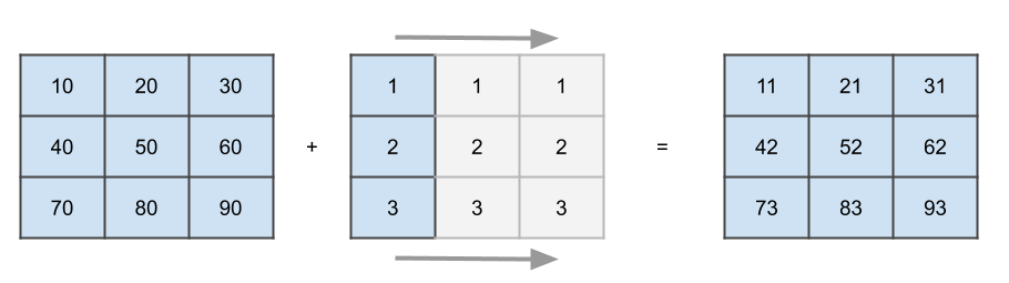
This is what happens on a conceptually level, NumPy will not actually increase the amount of memory occupied by your vector but simply loop over it to simulate the behavior. The broadcasting algorithm has only two rules:

1. The shapes will be compared element-wise from right to left (starting at the trailing dimension)
2. They are compatible if
   1. They are equal
   2. One of them is one

In the image above, it will discover that we are trying to add a (3,3) matrix with a (3,1) matrix (or vector), hence the second dimension of the smaller matrix will be rescaled to three.

Advanced Examples

Confusion Matrix

This is a task I once got during an interview, the goal is to design and implement a confusion matrix class. It should allow to adding observations on a running basis and calculate the confusion matrix on demand. Here I added an option to get a matrix with counts or a normalized version. The number of classes which can be observed is fixed upon instantiation.

As a short repetition, a confusion matrix summarizes all the observations in a (n, n) matrix, where n is the number of classes. An entry confusion_matrix[i, j] counts how many observations in class i were predicted as class j.

class ConfusionMatrix:
    def __init__(self, classes: int):
        self.confusion_matrix = np.zeros((classes, classes))
        
    def add_observations(self, predicted_labels: np.ndarray, true_labels: np.ndarray) -> None:
        for true_label, predicted_label in zip(true_labels, predicted_labels):
    		self.confusion_matrix[true_label, predicted_label] += 1

	def get(self, normalized: bool) -> np.ndarray:
        if normalized:
            # We assume no row is empty
            return self.confusion_matrix / np.sum(self.confusion_matrix, axis=1)[:, None]
        return self.confusion_matrix.astype(np.int32)
    
# Basic testing of the functionality
confusion_matrix = ConfusionMatrix(classes=2)
confusion_matrix.add_observations(np.array([1,1,0,0,0]), np.array([1,1,1,0,0]))
confusion_matrix.get(normalized=False)
array([[2, 0],
       [1, 2]], dtype=int32)
confusion_matrix.get(normalized=True)
array([[1.        , 0.        ],
       [0.33333333, 0.66666667]])

The tricky part is the get method, where we have to be careful not to return the original reference. However the astype(type) method creates a copy automatically and the calculation for the normalized case does so too. Unfortunately so far I have not come across a way to add elements more efficiently than in an explicit for loop in the add_observations method. Also there is an implicit assumption in the normalized case, namely that no row is empty, in case any row violates that, it will be filled with np.nan.

Gradient Calculation for the Mean Squared Error with Softmax

One of the trickiest calculations in NumPy I have ever implemented was the gradient calculation of the mean squared error function with a softmax in this previous post. This is the math for a single image or sample:

The sum is over \(n\), which is the number of classes we want to predict. Moreover there are the true labels \(\mathbf{y_T}\) which we will call target in the implementation, and the log probabilities from the network \(\mathbf{y}\) which we will call input. For the formula above they are assumed to have the shape (classes). As we need the probabilities for the calculation we will transform the input with the softmax layer \(\mathbf{s} = \text{softmax}(\mathbf{y})\) for the vector and reference an element of that vector by \(s_i\) in the math part. We will call this vector softmax = softmax_layer(input) in the code. The operation does not change the dimensions, it stays a vector of shape (classes).

We have seen above that NumPy offers fast summation over an arbitrary axis or dimension of a an array, but how can we use this in this case? By expanding the vector to a matrix and then reducing it with a sum operation. The matrix we would like to sum up over should look like this:

Then we can simply do np.sum(G, axis=1) to get the gradient. But calculating the individual terms in \(G\) is still not trivial, we need to split it up into three terms:

• The left side: \((s_i - y_{Ti})\) represented by the matrix \(L\)
• The middle: \(s_i\) represented by the matrix \(M\)
• The right side: \((\mathbb{1}_{i=1} - s_j)\) where \(j\) is the row number, represented by the matrix \(R\)

We will create a matrix with each individual term \(L, M, R\) and then use element wise multiplication \(*\) to create the product above. The final product is then:

With individual matrices

Now a pattern starts to emerge in the first two matrices, they repeat over the rows. This is great because we then can take the individual vectors and simply broadcast them along that axis using softmax[None, :] and target[None, :]. The last matrix is the difference between a diagonal matrix with element \(1\) and the softmax vector being broadcasted horizontally :

The softmax can be broadcasted horizontally using softmax[:, None]. For the diagonal matrix NumPy provides a method allowing us to spread elements over a the diagonal of a matrix: np.diag([1] * classes). Here it is simply an array of ones. Putting all of the above calculations together, we have a gradient calculation method for a single input:

def gradient_one_example(input: np.ndarray, target: np.ndarray) -> np.ndarray:
    classes = input.size
    softmax = softmax_layer(input)
    L = softmax[None, :] - target[None, :]
    M = softmax[None, :]
    R = np.diag([1] * classes) - softmax[:, None]
    G = (2.0 / classes) * L * M * R
    return np.sum(G, axis=1)

However in a real implementation we would need to process more than one example, the input and target would be of shape (batch_size, classes), for simplicity we keep the ideas from above and simply loop over the batch size.

def gradient(input: np.ndarray, target: np.ndarray) -> np.ndarray:
    batch_size, classes = input.shape
    gradient = np.zeros_like(input)
    for i in range(batch_size):
        gradient[i] = gradient_one_example(input[i], target[i])
    # The simple method already divides by classes
    return gradient / batch_size

The explicit loop is not optimal, we can still improve by delegating all the calculations to NumPy with some careful broadcasting. Only this time we will need to extend to three dimensions instead of two:

def gradient(input: np.ndarray, target: np.ndarray) -> np.ndarray:
    batch_size, classes = input.shape
    softmax = softmax_layer(input)
    L = softmax[:, None, :] - target[:, None, :]
    M = softmax[:, None, :]
    R = np.diag([1] * classes)[None, :, :] - softmax[:, :, None]
    G = 2.0 / (batch_size * classes) * L * M * R
    return np.sum(G, axis=2)

The resulting tensors are a bit harder to visualize due to the additional dimension, but the G matrix will be of shape (batch_size, classes, classes) before the summation. The changes are not too difficult:

• The softmax and target arrays in the L and M tensors, we simply broadcast along the second dimension instead of the first (the first being the batch size) using [:, None, :].
• The diagonal matrix needs to broadcast along the first or batch_size dimension to be compatible with the softmax, this is done using [None, :, :].
• The softmax in the R matrix needs to be stretched or broadcasted along the third dimension to replicate the same pattern as in the two dimensional case, this is done with [:, :, None].

The resulting gradient method has been compared with a PyTorch implementation in the test here and returns the same values.

Conclusion

First we saw the basics of NumPy arrays, how to create and manipulate them. Then we saw what vectorized computations are and why they are preferable to python implementations of the same operations. Lastly, we saw what broadcasting is and how to use it together with vectorization.

References

A list of resources used to write this post, also useful for further reading:

• Array Basics and Vectorized Computation chapter in the Python for Data Analysis book for an intro to NumPy and Vectorization

• Advanced NumPy chapter in the Python for Data Analysis book for details on Broadcasting

• Array Broadcasting in Numpy in the official NumPy documentation

• Blog post giving a similar introduction to Vectorization and Broadcasting with more examples

Comments

I would be happy to hear about any mistakes or inconsistencies in my post. Other suggestions are of course also welcome. You can either write a comment below or find my email address on the about page.