The goal of this post is to create the basic building blocks of a neural network from scratch. This means without using any PyTorch or Tensorflow library functionalities, but in the end the code should look as simple as when using them. This work is based on the fast.ai course called deep learning from the foundations which gives an introduction similar to this over multiple lectures. I highly recommended watching the entire course.

Even though the goal is to write a library, whenever a new concept is introduced we will also explore the accompanying mathematical part.

Basic concepts and notation

Readers familiar with the basic concepts and notation for neural networks may skip this section.

• Scalar: A scalar \(a \in \mathbb{R}\) is a single number. Usually denoted in lower case.

• Vector: A vector \(\mathbf{v} \in \mathbb{R}^n\) is a collection of \(n\) scalars, where \(n>0\) is an integer.

  \[\mathbf{v}=\begin{pmatrix} v_{1} \\ v_{2} \\ \vdots \\ v_{n} \\ \end{pmatrix}\]

  \(v_i\) is the \(i\)-th scalar value from the vector. A vector it is denoted in lowercase and bold.

• Matrix: A matrix \(A \in \mathbb{R}^{n \times m}\) for some integers \(n, m > 0\) is a collection of \(nm\) scalars or \(m\) \(n\)-dimensional vectors arranged as follows:

  \[A=\begin{pmatrix} a_{11} & a_{12} & \cdots & a_{1m} \\ a_{21} & a_{22} & \cdots & a_{2m} \\ \vdots & \vdots & \ddots & \vdots \\ a_{n1} & a_{n2} & \cdots & a_{nm} \\ \end{pmatrix}\]

  \(a_{ij}\) is a scalar value picked from the matrix at position \((i, j)\). By convention the first value in \(n \times m\) is the number of rows and the second the number of columns. A matrix is usually denoted in uppercase.

• Transposed Matrix: Transposing a matrix is an operation, suppose we have the same matrix \(A \in \mathbb{R}^{n \times m}\) as above, then \(A^T \in \mathbb{R}^{m \times n}\), the transposed matrix of \(A\) is defined as

  \[a^T_{ij} = a_{ji} \quad \forall i \in \lbrace 1, \dotsc, m \rbrace, j \in \lbrace 1, \dotsc, n \rbrace\]

  or more visually, we are “mirroring” the matrix along the diagonal:

  \[A^T = \begin{pmatrix} a^T_{11} & a^T_{12} & \cdots & a^T_{1n} \\ a^T_{21} & a^T_{22} & \cdots & a^T_{2n} \\ \vdots & \vdots & \ddots & \vdots \\ a^T_{m1} & a^T_{m2} & \cdots & a^T_{mn} \\ \end{pmatrix} = \begin{pmatrix} a_{11} & a_{12} & \cdots & a_{1n} \\ a_{21} & a_{22} & \cdots & a_{2n} \\ \vdots & \vdots & \ddots & \vdots \\ a_{m1} & a_{m2} & \cdots & a_{mn} \\ \end{pmatrix}\]

  Transposing a matrix has some interesting properties, such as \(A = (A^T)^T\), but we will not use those here.

• Row: When we want to access a row in a matrix \(A \in \mathbb{R}^{n \times m}\) we denote the \(i\)-th row as \(\mathbf{a_{i.}}\)

  \[\mathbf{a_{i.}} = \begin{pmatrix} a_{i1} & a_{i2} & \cdots & a_{im} \\ \end{pmatrix} \qquad i \in \lbrace 1, \dotsc, n \rbrace.\]

  As a row is a vector, we will denote it in bold.

• Column: When we want to access a column in a matrix \(A \in \mathbb{R}^{n \times m}\) we denote the \(j\)-th row as \(\mathbf{a_{.j}}\)

  \[\mathbf{a_{.j}}=\begin{pmatrix} a_{1j} \\ a_{2j} \\ \vdots \\ a_{nj} \\ \end{pmatrix} \qquad j \in \lbrace 1, \dotsc, m \rbrace.\]

  As a column is a vector, we will denote it in bold.

• Dot product: The dot product between two vectors \(\mathbf{a}, \mathbf{b} \in \mathbb{R}^n\) is defined as

  \[\mathbf{a} \cdot \mathbf{b} := \sum_{i=1}^n a_i b_i\]

• Linear function: A function \(f : \mathbb{R} \longrightarrow \mathbb{R}\) is linear if it is of the form

  \[f(x) = ax+b \qquad \qquad \text{for } a,b \in \mathbb{R}\]

  This is the most simple case where we have a real valued function. But this also applies for more complicated objects such as vectors or matrices.

• Mean: Let \(n \geq 1\) and \(x_1, \dotsc , x_n \in \mathbb{R}\), the mean of \(x_1, \dotsc , x_n\) is

  \[\overline{x} = \frac{1}{n}\sum_{i=1}^n x_i\]

• Variance: Let \(n \geq 1\), \(x_1, \dotsc , x_n \in \mathbb{R}\) and \(\overline{x}\) the mean that sequence. Then the variance of \(x_1, \dotsc , x_n\) is defined to be

  \[\sigma^2 = \frac{1}{n}\sum_{i=1}^n (x_i -\overline{x})^2\]

• Normal Distribution: The normal or Gaussian distribution \(N(\mu, \sigma^2)\) for \(\mu, \sigma \in \mathbb{R}\) has the density

  \[f(x) = \frac{1}{\sigma \sqrt{2\pi}} e^{-\frac{1}{2}\big(\frac{x-\mu}{\sigma}\big)^2}\]

  We call it the standard normal distribution if \(\mu =0\) and \(\sigma^2=1\). Some of the important properties are best seen visually:

  

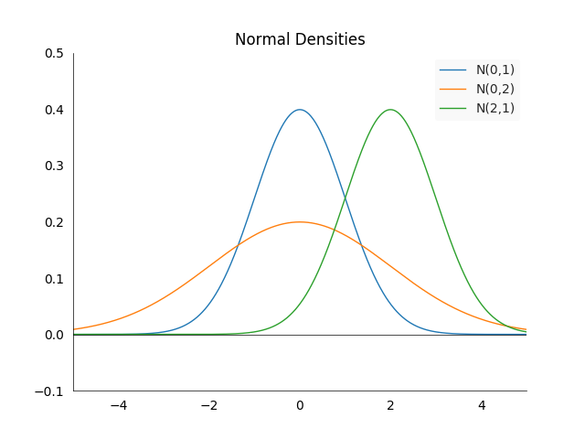
  The density is always centered at the mean \(\mu\) and symmetric around it. The larger \(\sigma^2\), the more spread out the density will be. \(67\%\) of the area under the density in between \(-\sigma^2\) and \(\sigma^2\). However the property we are going to use is not visible on the graph. Suppose we have two random variables \(X_1\) and \(X_2\) which follow normal distributions: \(X_1 \sim N(\mu_1, \sigma_1^2)\) and \(X_2 \sim N(\mu_2, \sigma_2)\). Then their sum is normally distributed again, i.e.:

  \[X_1 + X_2 \sim N(\mu_1+\mu_2, \sigma_1^2 + \sigma_2^2)\]

  This is not an obvious and also not a common property among random variables.

• Derivatives: If we have a function \(f: \mathbb{R} \longrightarrow \mathbb{R}\), then we will denote its derivative with respect to the input \(x\) as

  \[\frac{\partial f(x)}{\partial x} := \lim_{h \longrightarrow 0} \frac{f(x+h)-f(x)}{h}\]

• Directional Derivative: If \(f\) is a function which takes a vector as input, i.e. \(f: \mathbb{R}^n \longrightarrow \mathbb{R}\) and \(e_i \in \mathbb{R}^n\) the \(i\)-th basis vector, then we will call its derivative with respect to an input scalar \(x_i\) the \(i\)-th directional derivative:

  \[\frac{\partial f(\mathbf{x})}{\partial x_i} = \lim_{h \longrightarrow 0} \frac{f(\mathbf{x+e_i h})-f(\mathbf{x})}{h} \qquad \text{where } \mathbf{x + e_ih} = \begin{pmatrix} x_1 + 0 \\ x_2 + 0 \\ \vdots \\ x_i + 1h \\ \vdots \\ x_n +0 \\ \end{pmatrix}\]

• Gradient: At its core, the gradient is an operator which takes a differentiable function \(f\) and a vector \(\mathbf{x}\) in the input space of \(f\), and returns a vector in the same space as \(\mathbf{x}\). More formally if \(C^1(\mathbb{R}^n, \mathbb{R})\) is the space of all continuously differentiable functions from \(\mathbb{R}^n\) to \(\mathbb{R}\), then the gradient operator is defined as \(\nabla : C^1(\mathbb{R}^n, \mathbb{R}) \times \mathbb{R}^n \longrightarrow \mathbb{R}^n\) with

  \[\nabla f(\mathbf{x}) :=\begin{pmatrix} \frac{\partial f(\mathbf{x})}{\partial x_1} \\ \frac{\partial f(\mathbf{x})}{\partial x_2} \\ \vdots \\ \frac{\partial f(\mathbf{x})}{\partial x_n} \\ \end{pmatrix} \qquad f \in C^1(\mathbb{R}^n, \mathbb{R}), \mathbf{x} \in \mathbb{R}^n\]

  It is a vector of directional derivatives evaluated at point \(\mathbf{x}\).

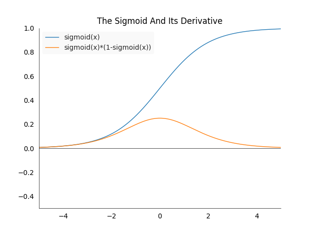
• Sigmoid: The sigmoid function \(\sigma : \mathbb{R} \longrightarrow (0,1)\), is defined as

  \[\sigma(x) := \frac{1}{1+\exp(-x)} = \frac{\exp(x)}{1+\exp(x)}\]

  It has the property that it maps any value to the open interval \((0,1)\), which is very useful if we want to extract a probability from a model. The derivative can be found by the following calculation

  \[\begin{align*} \frac{\partial \sigma(x)}{\partial x} &= \frac{\partial }{\partial x} \frac{1}{1+\exp(-x)} \\ &= \frac{\partial }{\partial x} (1+\exp(-x))^{-1} \\ &= -(1+\exp(-x))^{-2} \frac{\partial }{\partial x}(1+\exp(-x)) \\ &= \frac{\exp(-x)}{(1+\exp(-x))^2} \\ &=\frac{1}{1+\exp(-x)}\frac{\exp(-x)}{1+\exp(-x)} \\ &= \frac{1}{1+\exp(-x)}\frac{1 -1 +\exp(-x)}{1+\exp(-x)} \\ &= \frac{1}{1+\exp(-x)}\Bigg(\frac{1+\exp(-x)}{1+\exp(-x)} - \frac{1}{1+\exp(-x)}\Bigg) \\ &= \frac{1}{1+\exp(-x)}\Bigg(1 - \frac{1}{1+\exp(-x)}\Bigg) \\ &= \sigma(x)(1-\sigma(x)) \end{align*}\]

• Softmax: The softmax \(s: \mathbb{R}^n \longrightarrow (0,1)^n\) is the generalization of the sigmoid function. It is defined as

  \[s(\mathbf{x}) := \begin{pmatrix} \frac{\exp(x_1)}{\sum^n_{k=1} \exp(x_k)} \\ \frac{\exp(x_2)}{\sum^n_{k=1}\exp(x_k)} \\ \vdots \\ \frac{\exp(x_n)}{\sum^n_{k=1}\exp(x_k)} \\ \end{pmatrix} = \begin{pmatrix} s_1(\mathbf{x}) \\ s_2(\mathbf{x}) \\ \vdots \\ s_n(\mathbf{x}) \\ \end{pmatrix}\qquad \mathbf{x} \in \mathbb{R}^n\]

  Often we will omit \(\mathbf{x}\) for convenience and simply write \(s_i\) for a specific element in the vector.

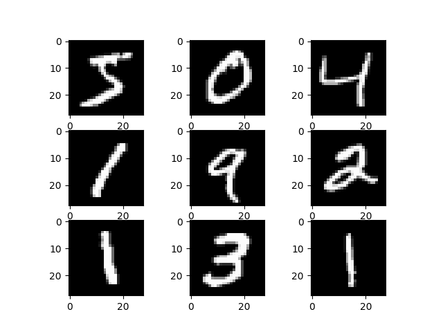
Data

We will use the most basic data for this task: MNIST. It consists of 28x28 images which display numbers from 0 to 9. To goal is tell which number is on which image.

The main data loading work is done in the fast.ai library, but this is of no concern to us as we want to focus on the neural network part and are happy to outsource data loading.

from fastai import datasets
import gzip
import pickle
import numpy as np
import typing
MNIST_URL='http://deeplearning.net/data/mnist/mnist.pkl'

def load_data() -> typing.Tuple[np.ndarray, np.ndarray, np.ndarray, np.ndarray]:
    path = datasets.download_data(MNIST_URL, ext='.gz')
    with gzip.open(path, 'rb') as f:
        ((x_train, y_train), (x_valid, y_valid), _) = pickle.load(f, encoding='latin-1')
    y_train, y_valid = index_to_one_hot(y_train), index_to_one_hot(y_valid)
    return x_train, y_train, x_valid, y_valid

The labels are loaded as a class label, for example class four will just be a \(4\), but we would like to have one hot encoded vectors, which are of the form \([0,0,0,1,0,0,0,0,0,0]\). The following method helps us transform the labels to vectors:

import numpy as np

def index_to_one_hot(index: np.ndarray) -> np.ndarray:
    max_elem, min_elem = np.max(index), np.min(index)
    n, classes = index.size, max_elem + 1 - min_elem
    one_hot = np.zeros((n, classes))
    one_hot[np.arange(n), index] = 1
    return one_hot

There is one big assumption in the method, namely that all classes are present in the data, you can see that in the line where we calculate the number of classes. This might not be suitable for cases where one class is extremely rare and does not appear in one of the sets.

Normalizing Data

So far we have just loaded the raw data from the files, however when feeding data to neural network it needs to be normalized to have mean zero and standard deviation one. This is very important as the they are sensitive to the input distribution, failure to do this will lead to unexpected behavior and most likely trainings which will not converge.

import numpy as np

def normalize(x: np.ndarray) -> np.ndarray:
    mean, std = x.mean(), x.std()
    return (x-mean)/std

We will see later what the effect of unnormalized data is in more detail, generally it will be important that the data keeps this distribution as it passes through the network.

Forward Pass

Matrix Multiplication

At the very basis of a lot of operations in neural networks is the matrix multiplication.

Formal Definition

Let \(A \in \mathbb{R}^{n \times m}\) and \(B \in \mathbb{R}^{m \times l}\) be two matrices. Then \(C \in \mathbb{R}^{n \times l}, C = A \cdot B\) is defined as

In words, each element of the resulting matrix \(C\) is the sum of the dot product of a row in \(A\) and a column in \(B\). Notice that the case where we multiply a matrix with a vector is just a special case of matrix multiplication with \(l=1\). We can write the above formula as

These formula are a bit hard to grasp at a first glance, let us do a small example to visualize the process of matrix multiplication.

A small example

Suppose we want to multiply two matrices \(A \in \mathbb{R}^{4 \times 3}\) and \(B \in \mathbb{R}^{3 \times 2}\). The resulting matrix \(C=AB\) will have the shape \(\mathbb{R}^{4 \times 2}\). Note that the resulting shape is the first dimension of the first matrix \(A\) and the second dimension of the second matrix \(B\).

Even after seeing the complete example, it might still be a bit mysterious how we arrived at the final numbers. After all the formula we defined above was for a single element. Hence lets have a look how we calculate the value of \(c_{31}\), the element of \(C\) in the third row and first column. The elements from \(A\) and \(B\) which we use for our calculations have been colored in blue and red, the result in green:

If we now apply the definition we get

Let us now write up this calculations in code.

In code

A straightforward way would be to simply translate the mathematical definition to code. Assuming that \(A\) and \(B\) are NumPy arrays with the proper shapes. We add an assert to check that the dimensions match.

import numpy as np

def matrix_multiplication(A: np.ndarray, B: np.ndarray) -> np.ndarray:
    n, m_a = A.shape
    m_b, l = B.shape
    assert m_a == m_b, f"Dimension mismatch for A an B: {m_a} != {m_b}"
    m = m_a
    C = np.zeros((n, l))
    for i in range(n):
        for j in range(l):
            for k in range(m):
                C[i,j] += A[i, k] * B[k, j]
    return C

However as this is an highly inefficient way of doing matrix multiplication in Python, it is best to delegate these computationally heavy calculations to optimized libraries, such as PyTorch or NumPy.

import numpy as np
    
def matrix_multiplication(A: np.ndarray, B: np.ndarray) -> np.ndarray:
    return A.dot(B)

Confusingly, the matrix muliplication in NumPy is called dot, writing A * B would do element wise multiplication.

Fully connected or linear layer

A fully connected or linear connects every input value with every output value. In most cases the input and output size is fixed by the data. We are looking at MNIST images with digits of size \(28 \times 28\) as inputs, it is quite natural to denote images as matrices. Hence we can denote them by \(X \in \mathbb{R}^{24 \times 24}\). Our output is constrained by the number of classes we want to predict. For MNIST there are digits from 0 to 9, or 10 different classes, therefore the output is a vector \(\mathbf{y} \in \mathbb{R}^{10}\). But which operation will transform an \(24 \times 24\) matrix to a \(10\)-dimensional vector, connecting every input value to every output value along the way?

The answer is that we need to flatten our input image to a \(784\)-dimensional vector \(\mathbf{x} \in \mathbb{R}^{784}\) and apply a matrix multiplication. A flattening operation takes every image row and simply concatenates them after each other. By performing this operation we lose spatial information, however as we connect the input with the output pixel-wise, this does not matter for for this case (this is not true when doing convolutions).

If we look at a single image and write the flattened matrix as a vector, then it has the shape \(X \in \mathbb{R}^{1 \times 784}\) and our output needs to be a matrix \(Y \in \mathbb{R}^{1 \times 10}\). Lets denote the matrix we are looking for as \(W\), our operation will be \(Y = XW\). By looking at the definition of the matrix operation we can see that \(n=1\), \(m=784\) and \(l=10\). We can now deduce the dimensions of \(W\) to be \(m \times l = 784 \times 10\), an object in \(\mathbb{R}^{784 \times 10}\). We can see this layer as a linear projection from the \(784\)-dimensional (input-)space into \(10\)-dimensional (output-)space:

Actually, any kind of neural network that does classification can be seen as a projection, of course in general neural networks are not linear. However as linear functions are quite strongly limited how they can represent data, we will try to get rid of that limit next. But first let us write up these insights in code.

import numpy as np

class Linear:
    def __init__(self, input_units: int, output_units: int):
        self.weights = np.random.randn(input_units, output_units)

    def __call__(self, input: np.ndarray):
        return matrix_multiplication(input, self.weights)

To create a layer for our MNIST case we would instantiate the class with linear_layer = Linear(784, 10) and call it with linear_layer(x). We need to chose initial values for our weights matrix, using zeros would be a bad choice as our output would be zero no matter the input. As a simple start we will use randomly generated values from a standard normal distribution. This means our matrix has mean zero and standard deviation of one, like our input. Why this is not a great idea will be shown later in the section on initialization.

Multiple Layers

For starters we can try adding more layers, that means instead of one multiplication we can do multiple ones in a row. Suppose we first want to reduce to \(50\) dimensions, and only then to \(10\). This is what we call a hidden layer in neural networks. In our case we would create matrices \(W_1 \in \mathbb{R}^{784 \times 50}\) and \(W_2 \in \mathbb{R}^{50 \times 10}\) to represent

And then do a concatenation \(f_2(f_1(X))\) to reduce the input to our desired size.

Concatenating linear functions

So does concatenating linear functions help us get non-linear functions? Unfortunately not. To see this consider the simple case of two linear functions \(f(x) = ax +b\) and \(g(x) = cx + d\) where \(a,b,c,d \in \mathbb{R}\), then if we concatenate these functions as suggested before we get

\(g(f(x)) = g(ax + b) = c(ax+b) + d = cax + cb + d = ex+f \quad e, f \in \mathbb{R}\).

Which is the definition of a linear function. The same happens when we do matrix multiplication, only the calculations get a bit more tedious because a lot more terms are involved. If we look closely at the equation above we see that we have been missing something else so far: the intercept.

Not having an intercept means that our function always has to go through the origin, i.e. \(f(0) = 0\). But it might be that we want to approximate functions which do not have this property, the answer is adding a vector with the output dimension. For the case of \(f_1\) above, we need \(\mathbf{b_1} \in \mathbb{R}^{50}\) and add it to the result: \(f_1(X) = XW_1 + \mathbf{b_1}\). Now we have a complete linear layer. Lets rewrite the class to reflect the change:

import numpy as np

class Linear:
    def __init__(self, input_units: int, output_units: int):
        self.weights = np.random.randn(input_units, output_units)
        self.bias = np.random.rand(output_units)
        
    def __call__(self, input: np.ndarray):
        return matrix_multiplication(input, self.weights) + self.bias

Non-linearities

The key to having more expressive networks is adding a non-linear function between linear layers. In the early days of deep learning people used sigmoid functions \(\sigma(x)\). However they have the unfortunate property that they will reduce the gradient when the values are not clustered around zero, this will lead to the so called vanishing gradient problem when training very deep networks. Nowadays it is standard to use a rectified linear unit, or ReLU:

The advantage here is that it is very simple to calculate, and the gradient will be unchanged for values above zero, and zero for anything else. It is not differentiable at \(z=0\), but this is not an issue in practice. The operation gets applied element-wise, that means we apply it for every scalar of the output of the matrix multiplication. The entire network with the above introduced functions \(f_1\) and \(f_2\) would now have the form

Note that we do not apply the non-linearity after the very last layer. In code the ReLU layer is quite simple:

import numpy as np

class ReLU():
    def __call__(self, input: np.ndarray):
    	return np.maximum(input, 0)

Here we can instantiate the object again with relu = ReLU() and call it with relu(x).

Initialization

So far we initialized our weight matrices with values drawn from a standard normal distribution. Assume that we want to build a network that is over a hundred layers deep, which is fairly standard these days if you want to get state of the art results. See for example the ResNet152, which is in the vision library of PyTorch. We can approximate this by doing a matrix multiplication for the same number of times. Let \(W_1, \dotsc, W_{152} \in \mathbb{R}^{512,512}\) be these \(152\) matrices. We initialize them randomly by drawing each value from a standard normal distribution \(N(0,1)\). Furthermore we also take a random input vector \(\mathbf{x} \in \mathbb{R^{512}}\), where each element is also drawn from a \(N(0,1)\) distribution. This mimics the input normalization we do for our data.

import numpy as np

x = np.random.randn(512)
np.mean(x)
-0.012377488357691202
np.std(x)
0.9713856958243533
for i in range(152):
    W = np.random.randn(512,512)
    x = W.dot(x)
np.mean(x)
-6.918073644685097e+203
np.std(x)
inf

The exact numbers you will get from running this code will vary, but the orders of magnitude will be similar. We should note here that NumPy is more generous with the numerical precision than PyTorch, if you do the same operations there, the result will be a vector full of nan (not a number). Intuitively the results is a bit strange, after all the numbers are equally likely to be positive or negative, and they are all clustered around zero (\(67\%\) of them will be between \([-1,1]\)). So why do they explode?

A mathematical explanation

To get a deeper understanding of what is happening inside these multiplications, let us look at the simpler case of one multiplication in the same setting as above, i.e. \(\mathbf{y} = W_1 \mathbf{x}\). We are especially interested in the distribution of the elements in the vector \(\mathbf{y}\), remember we would like them to follow a standard normal distribution \(N(0,1)\), the same as our input data. This is how one single element \(y_i\) of \(\mathbf{y}\) is calculated:

Each element in the weight matrix \(W\) independently follows a standard normal distribution, \(w_{ij} \sim N(0,1)\). If we ignore the \(x_j\) terms, we can see the term as a sum of \(n\) independent \(N(0,1)\) variables.

\(y_i\) is then also a normal variable and by a well known theorem we get that it follows also a normal distribution: \(y_i \sim N(0,n)\). However the variance is the sum of the individual variances because we have independence. We can transform it back to a standard normal distribution by dividing it by the square root of \(n\):

Going back to our original problem, the short analysis above suggests we could solve the problem of exploding values by multiplying each weight value \(w_{ij}\) by \(\frac{1}{\sqrt{n}}\). Let us define the new normalized weight matrix \(\hat{W}_1 = \frac{W_1}{\sqrt{n}}\) where we set \(n=512\) and get a new vector result vector \(\mathbf{\hat{y}}\) with values

Translating this into code, we only need to change one line to make our network more stable:

import numpy as np

x = np.random.randn(512)
np.mean(x)
-0.012377488357691202
np.std(x)
1.032536505693108
for i in range(152):
    W = np.random.randn(512,512) / np.sqrt(512)
    x = W.dot(x)
np.mean(x)
0.009774121752351837
np.std(x)
0.9994743773409233

Note that while running this code snippet multiple times, you will get quite diverse values for the standard deviation of \(x\) at the end. Mine varied from \(0.3\) to \(2.0\), however they will remain reasonably small. There is only one flaw in this analysis, so far we have neglected the key part of our network: the non-linearity.

Taking ReLU into account

How will the result change if we add ReLU layers after each multiplication? If we look at what ReLU does intuitively, it will move all the negative values to zero after every step. This means we will lose all the variation in the negative part of our output after each step, this will surely reduce our overall variation (or variance). This is exactly what we see in our experiment using a ReLU layer:

import numpy as np

x = np.random.randn(512)
relu = ReLU()
for i in range(152):
    W = np.random.randn(512,512) / np.sqrt(512)
    x = relu(W.dot(x))
np.mean(x)
4.5802235212737294e-24
np.std(x)
6.567280682740789e-24

The math is not as straightforward as in the previous case, but good insights can be gained from the paper by Kaiming. The solution is to multiply the square root of two into the normalization factor to increase the lost variation slightly. The resulting factor is \(\sqrt{\frac{2}{n}}\) or for our case \(\sqrt{\frac{2}{512}}\), which we can insert in our code to increase the variance:

import numpy as np

x = np.random.randn(512)
relu = ReLU()
for i in range(152):
    W = np.random.randn(512,512) * np.sqrt(2/512)
    x = relu(W.dot(x))
np.mean(x)
0.6635736242280306
np.std(x)
1.0063207498458

Note that we introduced a slight bias into the mean, it will generally be around \(0.5\), but this seems to be less of an issue. All the steps we have outlined above give us a certain guarantee that our network will produce reasonable output distributions at the initialization, however there is no restriction once we start training. Such restrictions can inserted into the network, the most popular one is called BatchNorm.

Loss

We now have all the tools to pass images through the network, but we still need to measure the results. The way we commonly do this are loss functions. In a previous post we saw why we generally use cross-entropy for classification and why mean squared error is a bad idea. However for illustration purposes we are still going to implement mean squared error and then cross-entropy afterwards. Let us define a general loss function as function taking two vectors and producing a positive scalar as loss:

The input to the loss will generally be the model output \(\mathbf{y} \in \mathbb{R}^n\), and target values \(\mathbf{y_T} \in \mathbb{R}^n\). We assume that the target will be represented as one-hot encoded vector. Note that one-hot encoded vectors are also discrete probability distributions. They fulfill the conditions that all elements are between zero and one and the sum of all elements is equal to one.

Mean Squared Error

The most basic loss is taking the L2 distance, or averaging the squared difference between the model output and the true label. We do this element wise and sum up the individual distances to get a scalar:

Note that we did not restrict the model output \(\mathbf{y}\) in any way. While our target will always be values which are either zero or one, our model output will not. In general this is a bad idea, one single output could completely dominate the loss by contributing a large value to it. However as we initialized our model to have outputs which are almost normally distributed around zero, so this should not happen in the beginning. And indeed, this approach, although theoretically unsound, will work surprisingly well. This is a general feature of neural networks, they are surprisingly resistant to small inconsistencies such as these, which can lead to many undetected bugs in a machine learning pipeline.

In code the entire loss becomes a single line

import numpy as np

class MSE:
    def __call__(self, input: np.ndarray, target: np.ndarray) -> np.ndarray:
        return np.mean(np.power(input-target, 2))

Mean Squared Error with Softmax

In order to restrict the model output to the same range as our labels, i.e. make it a probability distribution, we can use a softmax layer. The softmax output for the \(i\)-th element is defined as

Note that we will use \(s_i\) as the output for the loss function to make the equation more concise.

Although this approach sounds more reasonable in practice we will run into issues because the softmax layer will shrink our gradients if the values are not close to zero in the forward pass before the softmax layer. We will get to that in the gradient section.

For now let us have a look at the softmax layer implementation. We don’t simply do the calculation mentioned in the formula above, we are subtracting the maximum prediction for each vector first. This is done to for numerical stability and does not have an influence on the probabilities. We are taking advantage of the following softmax property:

This means the maximum value in the exponential function will be \(0\), and we do not risk the large values appearing after exponentiating the input.

import numpy as np

class Softmax:
    def __call__(self, input: np.ndarray) -> np.ndarray:
        input_max = np.max(input, axis=1)[:, None]
        input_exp = np.exp(input - input_max)
        return input_exp / np.sum(input_exp, axis=1)[:, None]

Moreover we are also taking advantage of a NumPy functionality called broadcasting. An detailed explanation would be out of the scope of this post, but in this case it helps us resizing the vector containing row wise maxima to a matrix.

The implementation of the MSES loss does not change significantly compared to the MSE. We simply need to create the softmax layer and use it before applying the loss function.

import numpy as np

class MSES:
    def __init__(self):
        self.softmax = Softmax()

    def __call__(self, input: np.ndarray, target: np.ndarray) -> np.ndarray:
        self.input, self.target = input, target
        return np.mean(np.power(self.softmax(input)-target, 2))

Cross-Entropy

Cross-entropy is a measure to compare two probability distributions, hence we have to restrict the model input to be a probability distribution as well. This is again done by applying a soft-max layer before the loss.

This expression will be positive as the input to the log will be restricted to the range of \([0,1]\) and we multiply all the elements by minus one. As our target vector is one-hot encoded, all the terms of the sum except for the one with the true label will become zero. So if the true label is \(k\), the loss will reduce to

The implementation is similar as with the MSES loss, however we only take the values into account where our target vector is not zero.

import numpy as np

class CrossEntropy:
    def __init__(self):
        self.softmax = Softmax()

    def __call__(self, input: np.ndarray, target: np.ndarray):
        self.input, self.target = input, target
        input_probabilities = self.softmax(input)
        return np.mean(-1*np.sum(np.log(input_probabilities[target > 0])))

We still take the mean because the loss will be summed over multiple predictions, or images, at once. Finally we have collected all the ingredients to do a forward pass and evaluate it, next will put them together.

Model

To put all the layers together and call them sequentially, we create a model class. Its task is to create a prediction y = model(x) form some input x.

import numpy as np

class Model:
    def __init__(self, layers: list):
        self.layers = layers

    def __call__(self, x: np.ndarray) -> np.ndarray:
        for layer in self.layers:
            x = layer(x)
        return x

Also, we need a function to calculate the accuracy of the predictions. We simply chose the index containing the maximum value to be the predicted index (or class). Note that the raw output of the model is not probabilities. But the softmax transformation will not change the ordering of the elements, as the exponential is a strictly increasing function. Hence there is no need to apply it.

import numpy as np

def calculate_accuracy(output: np.ndarray, target: np.ndarray) -> np.ndarray:
    return np.mean(np.argmax(output, axis=1) == np.argmax(target, axis=1))

Putting it all together is only a few lines, first we load the data and select the first 100 elements (or images). Next we create the loss function and the model. The model contains three layers, two linear and a ReLU in between them.

x_train, y_train, _, _ = load_data()
first_images = x_train[:1000]
first_targets = y_train[:1000]

loss = CrossEntropy()
model = Model([Linear(784, 50), ReLU(), Linear(50, 10)])

y = model(first_images)
loss_value = loss(y, first_targets)
accuracy = calculate_accuracy(y, first_targets)
loss_value, accuracy
2592.4592221138564 0.112

Afterwards we run the images through the network and evaluate the predictions on the loss and accuracy function. The results are not great, because we did not train the network yet. The accuracy is at 11%, which is what we would expect when making random guesses, which have on average a 10% change of being right. Next, we will look at how to update the network to improve the loss and accuracy.

Backward Pass

The backward pass consists of calculating the gradient from the loss function and passing it backwards through the layers, storing it inside each of them. Why we can do this so easily and in a relatively isolated form is due to the Backprop algorithm. Explaining this in detail would be a topic for another large post. After we stored the gradient updates in the network, they can be applied in the optimization step.

Remember that our loss function was a function from a vector to positive scalar: \(l : \mathbb{R}^n \times \mathbb{R}^n \longrightarrow [0, \infty)\). The gradient of a loss function will not map to a scalar anymore, the output will be a vector of the same size as the input, where the values can also be negative:

More specifically the gradient will be taken with respect to the input vector \(\mathbf{y}\) for a target vector \(\mathbf{y_T}\):

Each of the expressions inside the vector is a function which maps to a scalar. So for example if

Then the partial derivatives and the gradient with respect to \(x\) are

Note that the gradient depends on the input values of both of the vectors (as in example), this means we have to store them for each layer. Unfortunately the calculus becomes a bit more complicated when matrices are involved, such as in the linear layer.

Gradients and Back-Propagation

First we will calculate the gradients of various loss functions, and then we pass them as updates through the layers. Generally it is easier to first look at the gradients or partial derivatives in only one dimension with a single example. Then we can generalize to multiple dimensions and finally to multiple examples. Where the last step is generally an average or sum of the gradients per example.

Mean Squared Error

The MSE loss has a relatively straightforward update. Let us first suppose we do this for a case where we have one example and a one dimensional output \(y\), then this reduces to

If the output \(\mathbf{y}\) is a vector, then the same rule applies for every output dimension:

All the terms except for one become zero in each line. If we have \(m\) examples, then we take the average for each individual dimension

The indexes can become quite messy, but the principle should be clear. From now on we will assume that the last step is straightforward and will not explicitly mention it anymore.

We need to adapt the forward pass to store the the input and target values. Additionally we add the gradient method which will return the gradient for the last loss we calculated.

import numpy as np

class MSE:
    def __call__(self, input: np.ndarray, target: np.ndarray) -> np.ndarray:
        self.input, self.target = input, target
        return np.mean(np.power(input-target, 2))

    def gradient(self) -> np.ndarray:
        return 2.0 * (self.input - self.target) / np.multiply(*self.target.shape)

Note that the loss calculation is not strictly necessary to have a gradient. We nevertheless make them dependent by having stored the input and target values as attributes.

Mean Squared Error with Softmax

Let us do the same steps for the MSE with softmax. This will add an additional step to the derivative because we have to take the softmax into account. We start again with the simple case of a one dimensional function with one dimensional input:

How to calculate the derivative of the sigmoid is explained in the introduction. Note that as we normalized the input to a probability, the difference between the label and the output can no longer be larger than one. We see that the term is pretty similar to the the mean squared error but with an additional factor of \(\sigma(y)(1-\sigma(y))\). This factor will shrink the gradient considerably as the following plot shows.

In the best case the gradient will be shrunk by a factor of one fourth. This will slow the learning process down considerably as we will see during the tests. This factor is one of the reasons why we prefer cross-entropy for classification tasks.

Now on to the multi-dimensional case where the sigmoid is replaced by a softmax.

Unfortunately this time the sum does not disappear as before, the derivative of the inner function of \(( \cdot )^2\) does not disappear because the \(s_i\) depend on \(y_k\) for all \(k\). So what is the derivative of the softmax exactly? First we have to note that \(s : \mathbb{R}^n \longrightarrow \mathbb{R}^n\) is a function from a vector to a vector, so the derivative would be the a Jacobian matrix. However we only deal with \(s_i : \mathbb{R}^n \longrightarrow \mathbb{R}\), which is essentially the \(i\)-th output of the softmax function \(s\). As it returns a scalar, we can take the derivative w.r.t. to different input scalars. For example here the case with \(y_j\)

This calculation can then be inserted in the equations from before, with the twist that we can fix \(j\) for each row:

The above equations have been confirmed to be correct by Yoshua Bengio himself.

The implementation of the gradient calculation is more difficult here because of all these terms appearing in the gradient. With some careful broadcasting in NumPy we can avoid writing any loops and do all the work efficiently in a few lines:

import numpy as np

class MSES:
    def __init__(self):
        self.softmax = Softmax()

    def __call__(self, input: np.ndarray, target: np.ndarray) -> np.ndarray:
        self.input, self.target = input, target
        return np.mean(np.power(self.softmax(input)-target, 2))

    def gradient(self) -> np.ndarray:
        batch_size, classes = self.input.shape
        softmax = self.softmax(self.input)
        left_terms = softmax[:, None, :] - self.target[:, None, :]
        middle_terms = softmax[:, None, :]
        right_terms = np.diag([1] * classes)[None, :, :] - softmax[:, :, None]
        gradients = 2.0 / (batch_size * classes) * left_terms * middle_terms * right_terms
        return np.sum(gradients, axis=2)

Note that the last line is calculating the sum we also see in the gradient. The second last line is providing all the product terms needed for the summation. Before that we are only resizing the arrays among various dimensions to make the final calculation possible in two lines. If you are curious about how and why that works, there is a detailed explanation in this post.

Cross-Entropy

For cross-entropy we begin again with the easiest case where we have a binary classification problem, so our only parameter is a probability \(p\) and a label: true probability \(y_T\). For this case the cross entropy loss is defined as

As the label \(y_T\) is one hot encoded, it will be either zero or one. Which will zero out one of the two terms above. Suppose \(y_T=1\), then the loss turns into \(-\log(p)\) with derivative

The probability \(p\) will be the softmax \(s_i\). The general cross-entropy loss is defined as

As always \(\mathbf{y_T}\) is one hot encoded, hence only one term will remain, let’s call this the correct class \(c \in \lbrace 1, \dotsc n \rbrace\), it follows that \(y_{Tc}=1\). The loss is then reduced to \(l_{CE}(\mathbf{y}, \mathbf{y_T}) = -\log(s_c)\). The partial derivative with respect to \(y_j\) is

Or written it in the same vector notation we used above:

In other words, it will be \(s_j\) if \(j \neq c\) and \(s_c - 1\) for the true label \(c\). The implementation is straightforward as our gradient is the output of the softmax layer minus one where the ground truth is one.

import numpy as np

class CrossEntropy:
    def __init__(self):
        self.softmax = Softmax()

    def __call__(self, input: np.ndarray, target: np.ndarray):
        self.input, self.target = input, target
        input_probabilities = self.softmax(input)
        return np.mean(-1*np.sum(np.log(input_probabilities[target > 0])))

    def gradient(self) -> np.ndarray:
        gradient = self.softmax(self.input)
        gradient[self.target.astype(np.bool)] -= 1
        return gradient

Note that we need to create the softmax layer upon initialization and safe the input and output for the gradient calculations.

ReLU

In case of the intermediate layers there is a slightly different procedure to follow. They receive the gradient from the previous layer, which can be either a loss or another intermediate layer, store updates for their parameters and pass it on. In the case of the ReLU layer which represents the function \(ReLU(x) = \max(0,x)\) there are no parameters to adapt. The derivative of the ReLU layer is

Hence we set the gradient to zero where the output was zero and otherwise multiply by one, which means simply passing the gradient on. As the function is applied element wise there is no need to consider the multi-dimensional case any differently than above. Hence if \(\nabla_{\mathbf{y}}\) is the input gradient vector the output gradient vector \(\nabla_{\mathbf{x}}\) will be

We can translate that to code in one line:

import numpy as np

class ReLU():
    def __call__(self, input: np.ndarray):
        self.output = np.maximum(input, 0)
        return self.output

    def backward(self, gradient: np.ndarray):
        gradient[self.output == 0] = 0
        return gradient

The shape of the gradient will stay the same for this layer, just as the shape of the input remained the same in the forward pass.

Linear Layer

The case for the linear layer is slightly more complex for two reasons:

• The input and output size are not the same
• It contains parameters which need to be updated

Lets look at the first point, suppose that we have an input vector \(\mathbf{x} \in \mathbb{R}^n\), a weight matrix \(W \in \mathbb{R}^{m \times n}\) and a bias vector \(\mathbf{b} \in \mathbb{R}^m\) the output will then be \(\mathbf{y} = W\mathbf{x} + \mathbf{b} \in \mathbb{R}^m\). Note that this is a change in notation compared to above, it helps us write the multiplication more naturally. We will suppose that \(m < n\), i.e. the input vector is larger than the output vector. For each element \(y_i, i \in \lbrace 1, \dotsc m \rbrace\) in \(\mathbf{y}\) the output vector is obtained by

Note that \(b_i\) is outside the sum and only added once for the entire term. If we take the derivative w.r.t. to an arbitrary input \(x_k, k \in \lbrace 1, \dotsc, n \rbrace\), we get

What this tells us is that the directional derivative with respect to every input \(x_k\) will be non-zero in every in output \(y_i\), for indexes \(k \in \lbrace 1, \dotsc, n \rbrace\) and \(i \in \lbrace 1, \dotsc m \rbrace\). Let \(\nabla_{\mathbf{y}} \in \mathbb{R}^m\) denote the incoming gradient, or the derivative of the loss with respect to this layers output \(\nabla_{\mathbf{y}} = \frac{\partial l}{\partial \mathbf{y}}\). What we want to calculate is the gradient, or derivative of the input w.r.t. to the loss, i.e. \(\nabla_{\mathbf{x}} = \frac{\partial l}{\partial \mathbf{x}} \in \mathbb{R}^n\). If we look at a single term in the vector, we can simplify \(\nabla_{x_k}\) as follows

So to propagate the gradient back from the output to the input we multiply by the transposed of weight matrix \(W^T\). This will lead to a change dimension, the outgoing gradient will have the same shape as the input vector. We get

So far we have taken care of passing the gradient backwards, but what about the gradient with respect to the the parameters? This is what we will look at in the next section called optimization. For now the implementation of the above calculations is

import numpy as np

class Linear(Module):
    def __init__(self, input_units: int, output_units: int):
        self.weights = np.random.randn(input_units, output_units) * np.sqrt(2/512)
        self.bias = np.random.randn(output_units)

    def __call__(self, input: np.ndarray):
        return input.dot(self.weights) + self.bias

    def backward(self, gradient: np.ndarray):
        return gradient.dot(self.weights.transpose())

Note that here we do not need the input or output values to calculate the gradient, the weights are all that is needed for this layer.

Optimization

After creating the tools for forward and backwards passes, we have now all the necessary tools for the optimization step. There are various techniques for optimizing a function, however lots of them rely on the assumption the the function is convex, which is not the case for neural networks. Optimizing them is generally done with the gradient descent method, which in turn relies on a differentiable loss function (which all of our above losses are).

Gradient Descent

There are many explanations of gradient descent out there, here we will only do a quick review of the very basic optimization step used in this post. Suppose we have a differentiable function \(f : \mathbb{R} \longrightarrow \mathbb{R}\) and a starting point \(x_0 \in \mathbb{R}\), we would like to find the point \(x_s \in \mathbb{R}\) for which \(f(x_s)\) is minimal, i.e. \(f(x_s) \leq f(x) \: \: \forall x \in \mathbb{R}\). One way to do this is to find a sequence \((x_i)_{i \in \mathbb{N}} \in \mathbb{R}\) which converges to \(x_s\), or written differently \(x_s\) is the limit of \((x_i)\):

If we only have starting point \(x_0\), how do we find such a sequence? By doing gradient descent! The steps are iteratively and involve the gradient and a learning rate \(\gamma \in \mathbb{R}^+\)

Generally \(\gamma\) should be small, meaning less than one. The gradient points in the direction of the strongest increase in the function value. So if we go into the other direction then we should go towards a minimum, the minimum of the loss function we defined. To visualize this process, we take a simple example \(f\) and calculate its gradient:

This function will guide us to the point \(x_s = 2\), which is the only minimum with \(f(x_2) =1\). Setting the learning rate to \(\gamma = 0.1\) and the starting point to \(x_0 := 5\) gives us a sequence of the following values:

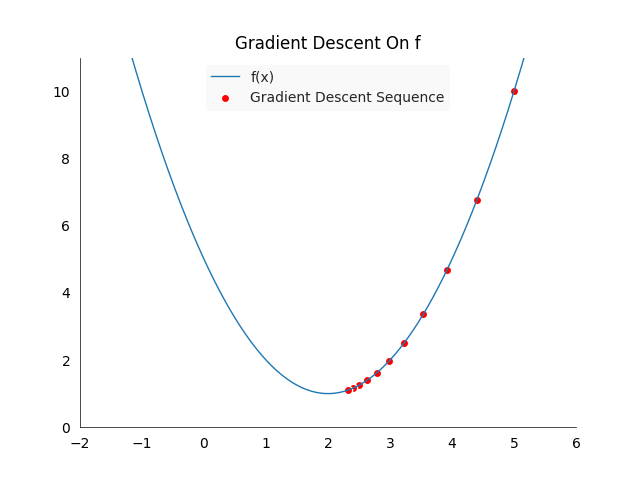
The above plot shows the first ten steps of the gradient descent algorithm, the points move from right to left, towards the minimum. The red points will cluster pretty quickly around the minimum of \(x_s = 2\). Gradient descent is guaranteed to converge to the global optima in the case of convex functions, such as in our example.

Unfortunately gradient descent does not give us any guarantee that we will find a global optima in the case of non-convex functions, we might get stuck in a local minimum. In practice there are many ways how we try to reduce the likelihood of ending up in a suboptimal solution, but for our problem here they won’t be necessary.

Linear layer

We can apply the same principle of gradient descent to the problem of optimizing a neural network, only now we won’t optimize a function \(f\) but our network for the loss \(l\). Most of the parts of the network we designed so far are static, except for the linear layer, which has two components which can be optimized:

• A weight matrix \(W\)
• A bias vector \(\mathbf{b}\)

For both we need to calculate the gradient with respect to their individual weights to update according to the gradient descent rule. Remember that we have as input the gradient vector \(\nabla_y\) and where the layer output is given by \(\mathbf{y} = W\mathbf{x} + \mathbf{b} \in \mathbb{R}^m\). First, let us look at the simpler part of updating the bias vector. For a single bias element \(b_k\), the derivative of the output with respect to \(b_k\) is

For the gradient with respect to the loss function we have to consider more terms

So for each element in the bias vector \(\mathbf{b}\) the gradient we need is simply the corresponding element in the incoming gradient vector \(\nabla_y\). If we denote the updated vector by \(\mathbf{b_{\text{new}}}\), then the gradient update is

That was not too difficult! We can do the same for the weight matrix, by looking first at a single element \(w_{kh}\) in the matrix. The gradient with respect to the output \(y_i\) is then

So for the \(k\)-th row the gradient depends on \(h\), otherwise it will be zero. The gradient with respect to the loss function obtained by the following calculation

The double sum simplifies nicely due to the two indicator function which effectively select one term each from the two sums. In simple terms, the gradient for the weight \(w_{kh}\) is the product of the \(h\)-th input element and the \(k\)-th incoming gradient element. How can we write this simple for the entire weight matrix? The answer is to see this as a matrix multiplication, but of two vectors. Remember that \(\nabla_{y} \in \mathbb{R}^m\), \(\mathbf{x} \in \mathbb{R}^n\) and \(W \in \mathbb{R}^{m \times n}\). We can also see the two vectors, \(\nabla_{y}\) and \(\mathbf{x}\), as matrix in \(\mathbb{R}^{m \times 1}\) and \(\mathbb{R}^{n \times 1}\) respectively. Transposing the gradient and multiplying the input with it gives us a matrix with the same size as the weight matrix:

Once we have the gradient the optimization step is again the generic gradient descent algorithm, for a new weight matrix \(W_{new}\) we do the update

In the implementation we will call \(\gamma\) learning rate. Note that we will need to store the input in the forward pass for the gradient update calculation. While the gradient calculation is done during the backward pass, the update is only applied when we call the update method with the learning rate.

import numpy as np

class Linear(Module):
    def __init__(self, input_units: int, output_units: int):
        self.weights = np.random.randn(input_units, output_units) * np.sqrt(2/512)
        self.bias = np.random.randn(output_units)
        self.weights_gradient = np.zeros((input_units, output_units))
        self.bias_gradient = np.zeros(output_units)

    def __call__(self, input: np.ndarray):
        self.input = input
        return input.dot(self.weights) + self.bias

    def backward(self, gradient: np.ndarray):
        self.weights_gradient = np.sum(self.input[:, :, None] * gradient[:, None, :], axis=0)
        self.bias_gradient = np.sum(gradient, axis=0)
        return gradient.dot(self.weights.transpose())

    def update(self, learning_rate: float):
        self.weights -= learning_rate * self.weights_gradient
        self.bias -= learning_rate * self.bias_gradient

The implementation is slightly different in the sense that we have to deal with multiple examples at once, this is where the sum term in the backward pass comes from. We also do not directly transpose the gradient, but let it broadcasting to the right size, this has the same effects but we only need to do an element-wise multiplication.

Finally we have everything to do complete forward and backward passes, plus an update step. First we need to update the model class to support the final two steps:

import numpy as np

class Model:
    def __init__(self, layers: list):
        self.layers = layers

    def __call__(self, x: np.ndarray) -> np.ndarray:
        for layer in self.layers:
            x = layer(x)
        return x

    def backward(self, gradient: np.ndarray):
        for layer in reversed(self.layers):
            gradient = layer.backward(gradient)

    def update(self, learning_rate: float):
        for layer in self.layers:
            layer.update(learning_rate)

It will take the gradient from the loss layer as input and propagate it backwards for each term. Then we can do one step each to see if the accuracy improves:

learning_rate, epochs, examples = 0.01, 30, 100
x_train, y_train, x_valid, y_valid = load_data()
multiple_images, multiple_targets = x_train[:examples], y_train[:examples]

loss = CrossEntropy()
model = Model([Linear(784, 50), ReLU(), Linear(50, 10)])

for i in range(epochs):
    y = model(multiple_images)
    loss_value, accuracy = loss(y, multiple_targets), calculate_accuracy(y, multiple_targets)
    gradient = loss.gradient()
    model.backward(gradient)
    model.update(learning_rate)

For readability reasons the loss and accuracy values are not printed, but have been plotted on an image. The cross-entropy loss has been reduced by a factor of \(100\) to fit it into the accuracy plot.

Overall we see what we would expect, the loss reduces sharply and the accuracy raises to a \(100\%\). Attentive observers will have seen that we train and test the network on the same images, this is not something one would usually do to make a serious model evaluation. However in this case it is useful to see if the network is capable of learning at all, which it is.

Tests

Whenever one writes code, it is a good habit to think of ways to validate it. This has many advantages, from discovering bugs to making sure the behavior of code stays the same over time. This is something I personally wish I had learned much earlier, it could have saved me countless days of wasted research efforts. Additionally it is in general quite hard to detect bugs in neural networks, they are so flexible that flaws can hide for quite a while. They might only manifest themselves by a slightly worse performance than expected, but discovering where the issue is in the pipeline will be quite time consuming.

In this section we will first write individual tests for layers and losses, and then do some quick end-to-end test to see if all the code fits together.

Unit

There are many ways to test the implementation of these basic building blocks, we could come up with examples and see if the results look as we expect or test against a reference implementation. The latter is what is done here, specifically we will test results against PyTorch implementations of the same layer.

Because minor imprecisions in numerical computation we will only test if the results are “close enough”, i.e. if the do not differ by more than a certain tolerance value. Here is a utility method which test if a tensor is close to zero for all elements:

import numpy as np

def assert_tensor_near_zero(tensor: np.ndarray, tol=1e-3) -> None:
    assert np.all(np.abs(tensor) < tol), f"Not zero: {tensor}"

There are some more technicalities to take care of, for example to conversion from torch tensors to NumPy arrays in an automated fashion, for this there are wrapper classes.

Testing a loss

Lets have a look how to test the cross-entropy loss. Firstly, we create the PyTorch version, a random input and target matrix. Then we test the loss when passing the input through our and the PyTorch version, they need to match by a certain tolerance threshold.

import torch
import numpy as np

def test_cross_entropy() -> None:
    batch_size, features = 3, 5
    torch_cross_entropy = torch.nn.CrossEntropyLoss()
    cross_entropy = ClassificationLossWrapper(CrossEntropy)

    input = torch.randn(batch_size, features, requires_grad=True)
    target = torch.empty(batch_size, dtype=torch.long).random_(features)
    # Forward loss
    loss = cross_entropy(input, target, classes=features)
    torch_loss = torch_cross_entropy(input, target)
    assert_tensor_near_zero(to_numpy(torch_loss) - loss)
    # Check gradient
    torch_loss.backward()
    torch_gradient = input.grad
    gradient = cross_entropy.gradient()
    assert_near_zero_tensor(to_numpy(torch_gradient)-gradient)

Secondly we propagate the loss backwards and test if the gradient from both layers are close. Note that in PyTorch the gradient is stored in the input variable, and is not a return value as in this implementation of loss functions.

Testing a layer

Testing a layer is slightly more complicated for a couple of reasons:

• Layers have parameters which need to be the same (in this case weight and bias)
• Have three functionalities to test: forward pass, backward pass, parameter update
• Need to be given a gradient, which means we have to involve a loss function (or invent a gradient)

Here we test the linear layer, forward and backward pass. To ensure the same parameters we copy the weight and bias the of the PyTorch layer to ours. After the forward pass we check if the results are the same. For readability, the code is split into two parts

import torch
import numpy as np

def test_linear():
    batch_size = 3
    in_features = 768
    out_features = 50
    torch_linear = nn.Linear(in_features=in_features, out_features=out_features)
    linear = LayerWrapper(Linear, input_units=in_features, output_units=out_features)
    input = torch.randn(batch_size, in_features, requires_grad=True)
    
    # Forward pass, to ensure same operation we copy weight and bias
    linear.update_attribute("weight", to_numpy(torch_linear.weight.T))
    linear.update_attribute("bias", to_numpy(torch_linear.bias))
    assert_tensor_near_zero(to_numpy(torch_linear(input)) - linear(input))

To test the backward pass we need to use a loss function to create a gradient. Which one we use is not important, it just needs to return a non-zero gradient. Here we use the MSE. Note that as a intermediate step, we also test that the two calculated losses correspond, this helps us detect problems at an earlier stage. There is also a check that the gradients, which update the parameters, are the same.

    # Backward pass, losses
    torch_loss = nn.MSELoss()
    loss = RegressionLossWrapper(MSE)
    # Backward pass, loss calculation and check
    target = torch.randn(batch_size, out_features)
    torch_loss_output = torch_loss(torch_linear(input), target)
    torch_loss_output.backward()
    loss_output = loss(torch.from_numpy(linear(input)), target)
    assert_tensor_near_zero(loss_output - to_numpy(torch_loss_output))
    
    # Backward pass, gradient pass
    gradient = linear.backward(torch.from_numpy(loss.gradient()))
    torch_gradient = input.grad
    assert_tensor_near_zero(to_numpy(torch_gradient) - gradient)
    # Backward pass, weight gradient
    torch_weight_gradient = torch_linear.weight.grad.T
    weight_gradient = linear.get_attribute("weight_gradient")
    assert_tensor_near_zero(to_numpy(torch_weight_gradient) - weight_gradient)
    # Backward pass, bias gradient
    torch_bias_gradient = torch_linear.bias.grad
    bias_gradient = linear.get_attribute("bias_gradient")
    assert_tensor_near_zero(to_numpy(torch_bias_gradient) - bias_gradient)

What is not done at this point is testing the update method, however this is only adding two attributes which we already know are correct: the parameters and their gradient.

End to end

For a quick end-to-end test we can run three different training runs, with the same network architecture and hyper-parameters but a different loss each. For all three the learning rate was constant at \(0.5\) over the entire training duration. The performance was relatively stable when making the learning rate an order of magnitude larger or smaller. However one could always fine tune it to make specific losses work better.

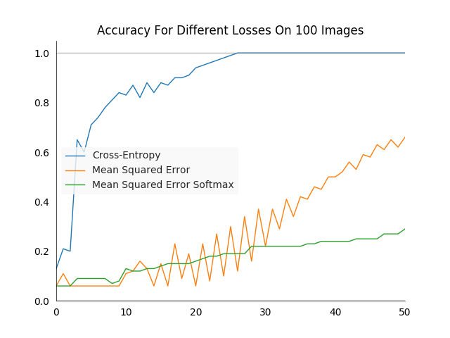
As expected, the cross-entropy loss performs best, while the network optimized on the MSES learns rather slowly.

Conclusion

We saw some of the major building blocks of a neural network: layers and losses. For each part there was a theoretical motivation followed by an implementation in Python. The two main phases of neural network training, the forward and backward pass were described for each component. In the end we wrote tests to verify the functionality.

References

All the code in this post can be found in a cleaned up version in my github repository called NeuralnetworkFromScratch.

A list of resources used to write this post, also useful for further reading:

• fast.ai course - Part 2: Deep Learning from the Foundations for a great introduction in general

  • Lesson 1 code for matrix multiplication
  • Lesson 2 code for forward and backward passes
  • Lesson 2b code for initialization

• Deep Learning book by Goodfellow, Bengio and Courville

  • Chapter 6 for fully connected layers, ReLU, back-propagation, MLP training

• Matrix multiplication Wikipedia

• Matrix transposition Wikipedia

• Dot product Wikipedia

• Linear function Wikipedia

• Fully connected layer Wikipedia

• Gradient Wikipedia

• Gradient descent Wikipedia

• Notes on Weight Initialization for Deep Neural Networks for a more detailed explanation on initialization

• How to initialize deep neural networks? for a good summary of the two initialization papers

• Gradient of a Matrix Matrix multiplication blog post on gradient calculations with multiple samples

• Derivative of the sigmoid function for a in detail calculation

• Derivative of the softmax function for an excellent explanation of the softmax and its derivative

• Derivative of MSE with softmax for the calculation of the loss

• CS231n: Convolutional Neural Networks for Visual Recognition for a Standford class introducing neural networks

Comments

I would be happy to hear about any mistakes or inconsistencies in my post. Other suggestions are of course also welcome. You can either write a comment below or find my email address on the about page.