This post are my lecture notes from watching the first six episodes of the excellent DeepMind x UCL Deep Learning Lecture Series 2020. I recommend to watch them in full, if you have the time. They cover a broad range of topics:

1. Introduction to Machine Learning and AI
2. Neural Networks Foundation
3. Convolutional Neural Networks for Image Recognition
4. Advanced Models for Computer Vision
5. Optimization for Machine Learning
6. Sequences and Recurrent Networks

While I tried to summarize the talk and the speaker as closely as possible, I did not aim to capture every detail. Sometimes I have added some remarks if parts of the lecture did not seem clear or some background information was useful for understanding the talk better.

Episode 1 - Introduction to Machine Learning and AI

01 - Solving Intelligence - 3:37

What is intelligence? Intelligence measures an agent’s ability to achieve goals in a wide range of environments. Or more technically we can define intelligence as

\[\Upsilon(\pi) := \sum_{\mu \in E} 2^{-K(\mu)}V^{\pi}_{\mu}\]

Where

• \(\Upsilon(\pi)\) is the universal intelligence of agent \(\pi\).
• \(\sum_{\mu \in E}\) is the sum over all environments \(E\)
• \(K(\mu)\) the Kolmogorov complexity function, a complexity penalty. Note that \(2^{-K(\mu)}\) becomes smaller for more complex environments, this measure gives more weight to simple tasks.
• \(V^{\pi}_{\mu}\) is the value achieved in environment \(\mu\) by agent \(\pi\).

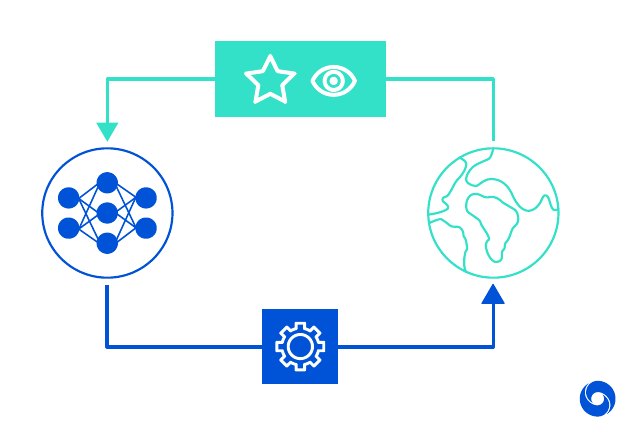
For more details you can read the original paper, the above formula can be found on page 23. This formula can easily be applied inside the reinforcement learning framework, where an agent interacts with the environment and receives rewards. The image below visualizes the concept in a very abstract way, the agent (left) interacts with the world (right) by giving it instructions (bottom) and receiving updates (reward, state).

Why did DeepMind choose games to solve intelligence?

1. Microcosms of the real world
2. Stimulate intelligence by presenting a diverse set of challenges
3. Good to test in simulations. They are efficient and we can run thousands of them in parallel, they are faster than real time experiments
4. Progress and performance can be easily measured against humans.

There is another talk where Demis Hassabis explains in more detail the reasoning of why DeepMind chose to solve games first.

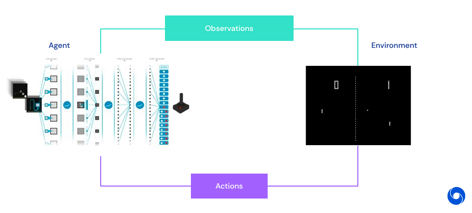
The above image visualizes the reinforcement learning feedback loop in games. Large parts of the agent consist of neural networks, using deep learning. Why is Deep Learning being used now?

• Deep Learning allows for end-to-end training
• No more explicit feature engineering for different tasks
• Weak priors can be integrated in the architecture of the network (such as in convolutions, recurrence)
• Recent advances in hardware and data
  • Bigger computational power (GPUs, TPUs)
  • New data source available (mobile devices, online services, crowdsourcing)

02 - AlphaGo and AlphaZero - 15:20

AlphaGo bootstraps from human games in Go by learning a policy network from thousands of games. Once it has weak human level it stars learning from self-play to improve further.

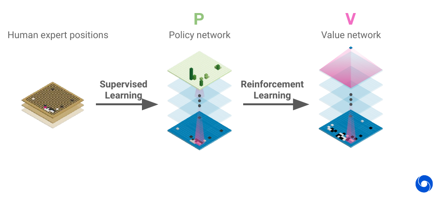
The policy network makes the complexity of the game manageable, you can do roll-outs by selecting only promising plays. The value network allows to reduce the depth of roll-outs by evaluating the state of the game at an intermediate stage.

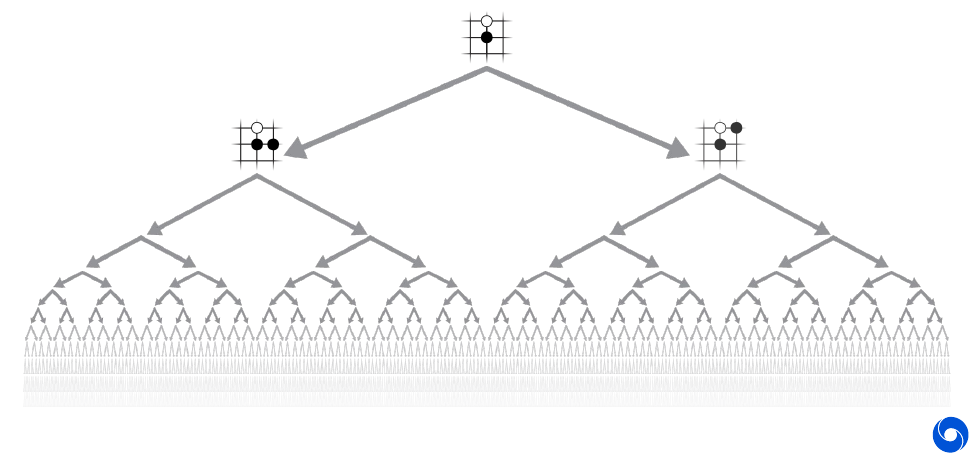
AlphaGoZero: Learns from first principles, starts with random play and just improves with self-play. Zero refers to zero human domain specific knowledge (in Go).

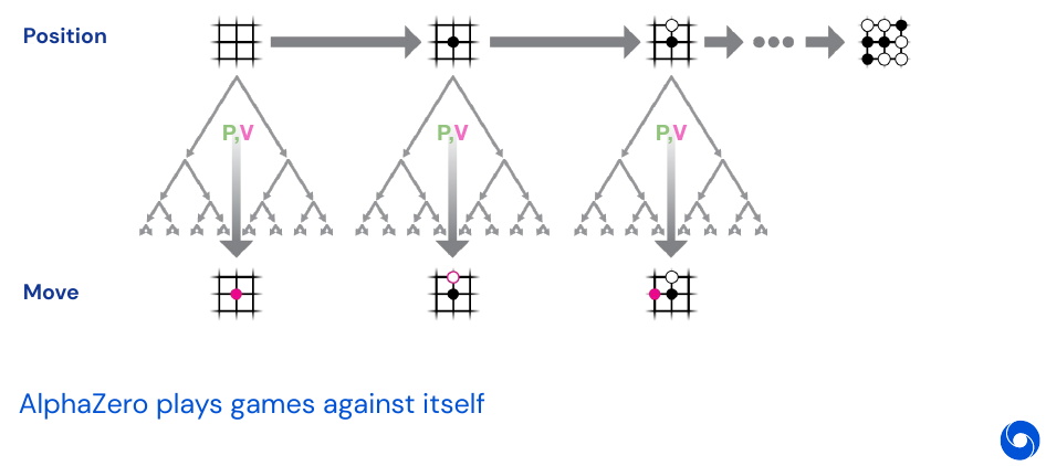
AlphaZero: Plays any 2-player perfect information game from scratch. It was also tested on Chess and Shogi, which is Japanese chess. Achieves human or superhuman performance on all of them. The way this works is to train a policy and value network, and then play against itself for hundred thousand plays. Then a copy of the two networks learns from that generated experience, once the new copy wins 55% of the games against the old version, the data generation process starts over.

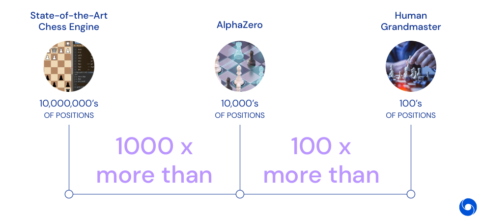
An interesting part of the lecture is that the amount of search an agent does before making a decision in chess. The best humans look at 100s of positions, AlphaZero looks at 10’000s of positions and a state-of-the art Chess engine looks at 10’000’000 of positions. This means the network allow for better data efficiency by selecting only promising plays to explore. AlphaZero beats both, humans and state-of-the-art Chess engines. AlphaZero also rediscovers common human plays in chess, and discards some of them as inefficient.

Conclusions about AlphaZero:

• Deep Learning allows to narrow down the search space of complex games
• Self-Play allows for production of large amounts of data which is necessary to train deep networks
• Self-Play provides a curriculum of steadily improving opponents
• AlphaZero is able to discover new knowledge and plays in the search space

03 - Learning to Play Capture the Flag - 32:21

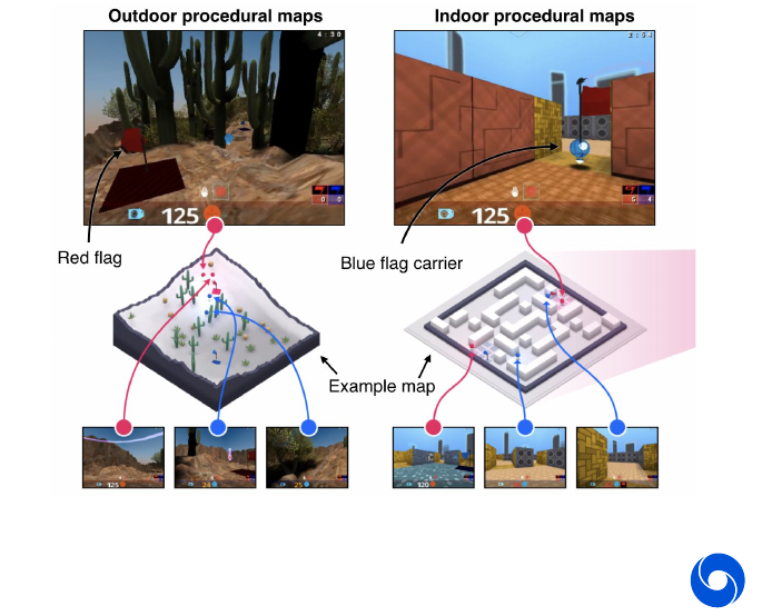
Capture the flag is a multi-agent game which is based on Quake III arena. Agents play in teams of two against each other and need to coordinate. The maps are procedurally generated, in indoor and outdoor style. A team can only score if their flag has not been captured by another team, this leads to a complex reward situation.

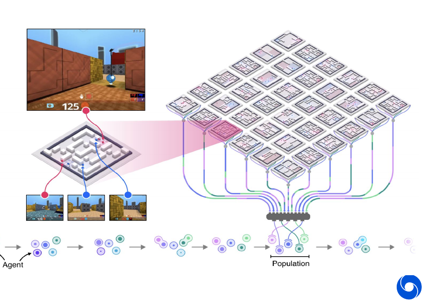
Here an entire population of agents are trained, a game is played by bringing multiple agents together. Each of them will only have access to his individual experience. There is no global information as in the previous cases. The population of agents serve two purposes:

• Diverse teammates and opponents, naive self-play leads to a collapse
• Provides meta-optimization of agents, model selection, hyper-parameter adaption and internal reward evolution

Achieves superhuman performance and easily beats baseline agents. The agent was evaluated in a tournament playing against and with humans. Humans can only beat them when their teammate is an agent. Surprisingly humans rated the FTW agent as the most collaborative.

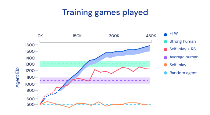
Agents develop behavior also found in humans, such as teammate following and base camping. Different situations of CTF can be visualized in the neural network by applying t-SNE to the activations.

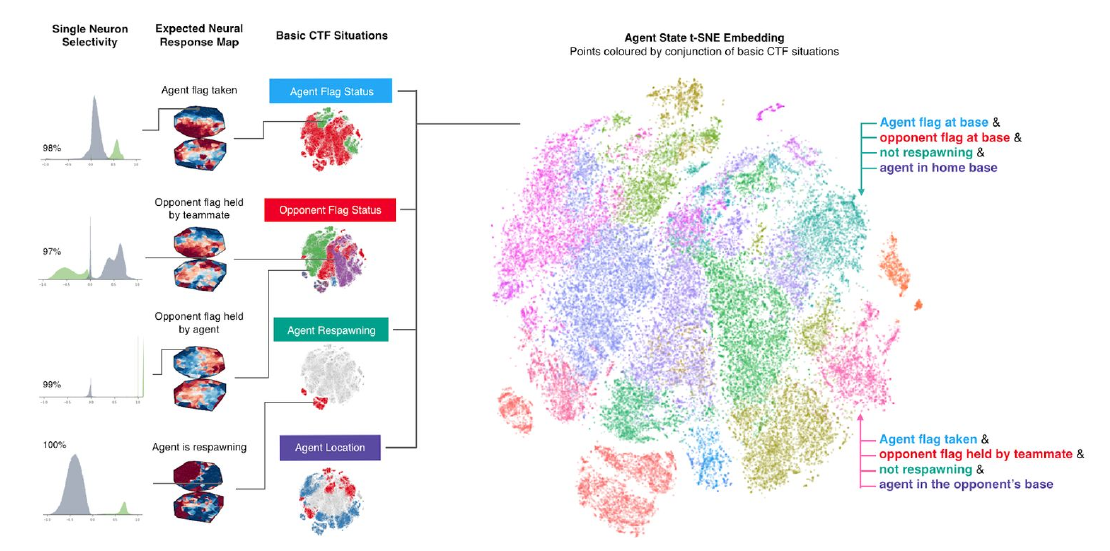
Conclusion:

• This shows that Deep Reinforcement learning can generalize to complex multi-player video games
• Populations of agents enable optimization and generalization
• Allows for understanding of agent behavior

04 - Beyond Games: AlphaFold - 41:13

Proteins are fundamental building blocks of life. They are the target of many drugs and are like little bio-mechanic machines. The shape of proteins allows to make deductions about their functions. The goal is to take as input a amino acid sequence and predict a 3D structure, which is a set of atom coordinates.

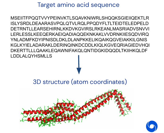
The problem is parametrized as follows:

• Predict the coordinates of every atom, especially the ones of the backbone
• Torsion angles \((\Psi, \Phi)\) for each residue are a complete parametrization of the backbone geometry
• There are \(2N\) degrees of freedom for chains of length \(N\)

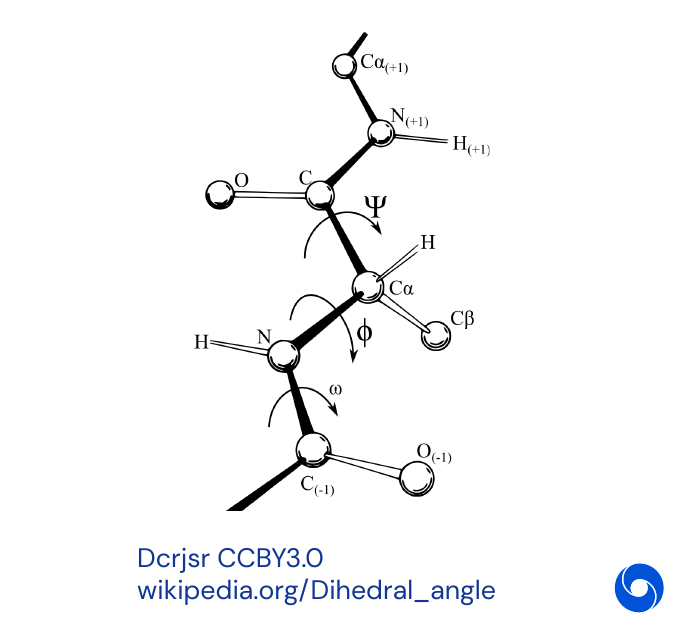
Levinthal’s Paradox says that despite the astronomical number of possible configurations, proteins fold reliable and quickly to their native state in nature. Finding the structure usually takes 4 years of human work, despite this there is a database of 150’000 entries available. This is not as much as in other domains (such as speech), but allows for Deep Learning to be applied.

The model takes a protein sequence as input to a neural network consisting of 220 deep dilated convolutional residual blocks, and predicts a map of pairwise distances plus angles. Then gradient descent is run on the resulting score function to obtain a configuration estimate.

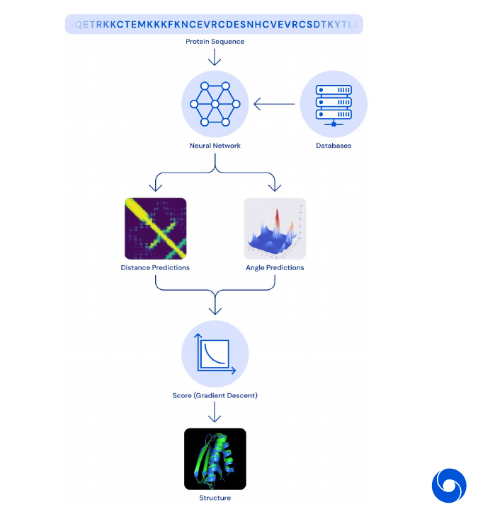
The whole system was evaluated on the CASP13 competition against other world class researcher on unseen data and achieved first place.

Conclusion:

• Deep Learning based distance prediction gives more accurate predictions of contact between residues …
• … but accuracy is still limited and only the backbone can be predicted. The side chains still rely on an external tool
• Work builds on decades of work by other researchers
• Deep Learning can deliver solutions to science and biology

05 - Overview of Lecture Series - 55:46

This part gives a quick overview of what will be discussed in the lecture series

1. Introduction to Machine Learning and AI
2. Neural Networks Foundation
3. Convolutional Neural Networks for Image Recognition
4. Vision beyond ImageNet - Advanced models for Computer Vision
5. Optimization for Machine Learning
6. Sequences and Recurrent Networks
7. Deep Learning for Natural Language Processing
8. Attention and Memory in Deep Learning
9. Generative Latent Variable Models and Variational Inference
10. Frontiers in Deep Learning: Unsupervised Representation Learning
11. Generative Adversarial Networks
12. Responsible innovation

Question Session - 1:13:08

What are the limits of Deep Learning?

• Lack of data efficiency
• Energy consumption of by computational systems
• Common sense, adapt quickly to new situations in an environment

Is autonomous driving AI complete?

• Probably needs more than reinforcement learning simulations only. Add physical simulations and multi-agent systems.

My Highlights:

• Definition of intelligence
• T-SNE view of how policy functions cluster

Episode 2 - Neural Networks Foundations

01 - Overview - 3:59

Deep Learning has been made possible by advances in parallel computation (important for matrix multiplication) and larger data sets. In general Deep Learning is not easy to define, an attempt from Yann LeCun:

“DL is constructing networks of parameterized functional modules & training them from examples using gradient-based optimization.”

We can see Deep Learning as a collection of differentiable blocks which can be arranged to transform data to a specific target.

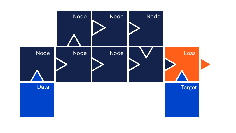
02 - Neural Networks - 9:17

An artificial neuron is losely inspired by real neurons in human brains. However the goal of an artificial neuron is to reflect some neurophysiological observation, not to reproduce their dynamics. One neuron is described by the equation

\[\sum_{i=1}^d w_i x_i + b \qquad d \in \mathbb{N}, w_i, x_i, b \in \mathbb{R}\]

and can be seen as a projection on a line.

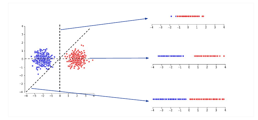
A linear layer is a collection of artificial neurons. In machine learning linear really means affine. We also call neurons in a layer units. Parameters are often called weights. These layers can be efficiently parallelized and are easy to compose.

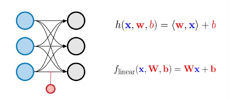
In order to make them non-linear, they are combined with sigmoid activation functions. We call them non-linearities, they are applied point-wise and produce probability estimates.

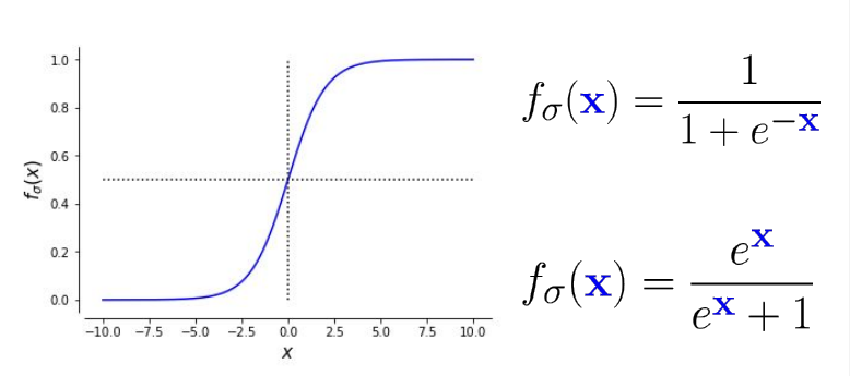
As mentioned in the puzzle above, we also need a loss function. It is often called negative log likelihood or logistic loss.

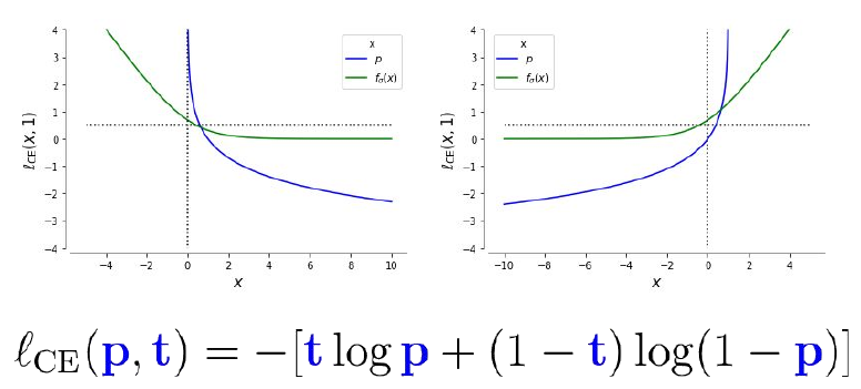
These components allow us to create a simple but numerically unstable neural classifier, because the gradient can vanish through some of these layers. We can see the gradient magnitude as amount of information that flows through a model.

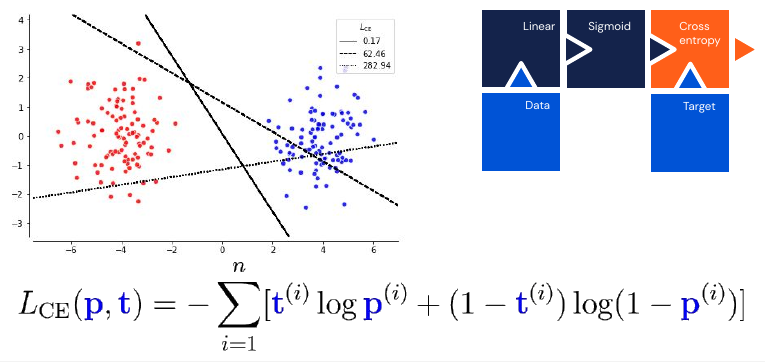
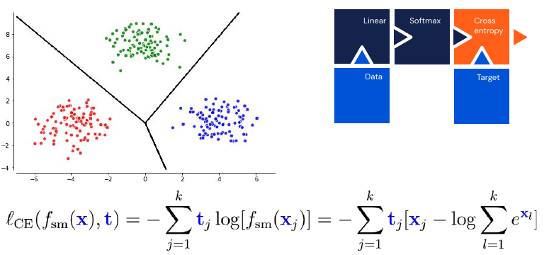
The above model is equivalent to a logistic regression. It is also additive over samples, which allows for efficient learning. We can generalize the sigmoid to \(k\) classes, this is called a softmax:

\[f_{sm}(\mathbf{x}) = \frac{e^{\mathbf{x}}}{\sum^k_{j=1} e^{\mathbf{x}_j}} \quad \mathbf{x} \in \mathbb{R}^k\]

It has the additional advantage of being numerically stable when used in conjunction with a Cross-Entropy loss. This is equivalent to a multinomial logistic regression model. However softmax does not scale well with the number of classes (if you have thousands of classes).

Surprisingly often high dimensional spaces are easy to shatter with hyperplanes. For some time this was used in natural language processing under the name of MaxEnt (Maximum Entropy Classifier). However it can not solve some seemingly simple tasks as separating these two classes (or can you draw a line to separate them?).

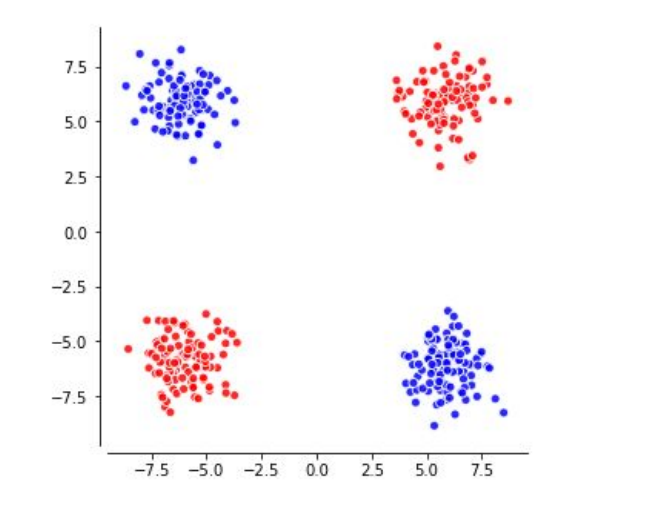
To solve the problem above, we need a hidden layer which projects the group of four points into a space where they are linearly separable (top left of the image).

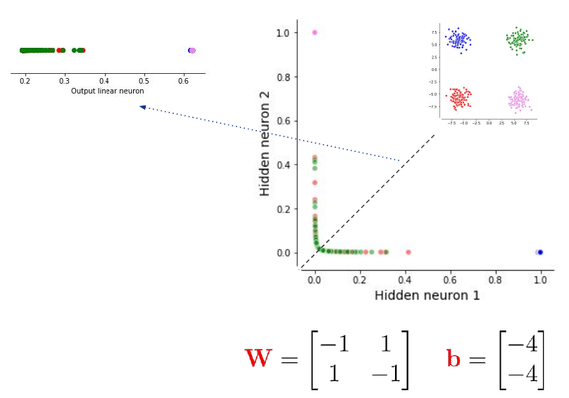
The hidden layer allows us to bend and twist the input space and finally apply a linear model to do the classification. We can achieve this with just two hidden neurons. To play around with different problems and develop some intuition go to playground.tensorflow.org.

One of the most important theoretical results for neural networks it the Universal Approximation Theorem:

For any continuous function from a hypercube \([0,1]^d\) to real numbers, and every positive epsilon, there exists a sigmoid based, 1-hidden layer neural network that obtains at most epsilon error in functional space.

This means a big enough network can approximate, but not necessarily represent, any smooth function. Neural networks are very expressive! This theorem can be slightly generalized to:

For any continuous function from a hypercube \([0,1]^d\) to real numbers, non-constant, bounded and continuous activation function f, and every positive epsilon, there exists a 1-hidden layer neural network using f that obtains at most epsilon error in functional space.

However these theorems tell us nothing about how to learn, or how fast we can learn those functions. The proofs are just existential, they don’t tell us how to build a network that has those properties. Another problem is that the size of the networks grows exponentially.

Remark: Considering that this theorem is for bounded activation functions, how does ReLU fit into the universal approximation theorem? It does not apply to that case. Most of the modern neural network use ReLU as non-linearity.

What is the intuition behind the Universal Approximation Theorem? We want to approximate a function in \([0,1]\) using sigmoid functions, then we can combine two of them, red and blue to get a bump (orange):

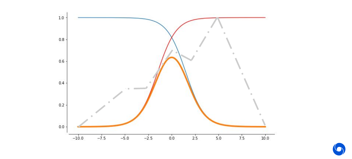
The more neurons we add, the more of these bumps we can get. The closer we can approximate the function. In the example below we use six neurons to approximate the function and can get already close. Intuitively it should be clear that the more neurons we use, the closer we can approximate the target function (grey) with the sum of our bumps (orange).

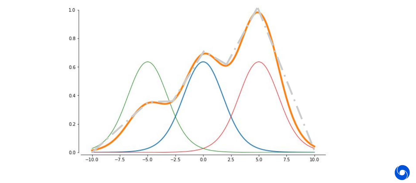
The theorem confirms the intuition that we can get arbitrarily close to any target function by simply using more of these bumps.

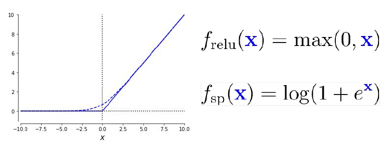
In practice we often do not use sigmoid but rectified linear units (ReLU) as activation functions. It has the advantage that the derivative does not vanish in the right side. However it can lead to ‘dead’ neurons which only output zero, due to this property careful initialization is necessary. Even though the function is not differentiable at zero, this is not an issue in practice.

Our overall goal is always to make the problem linearly separable in the last layer. In general is it more beneficial to create a wider than a deeper network? The question was answered in this paper, expressing symmetries and regularities is much easier with a deep than a wide network. The number of linear regions grows exponentially with depth and polynomially with width.

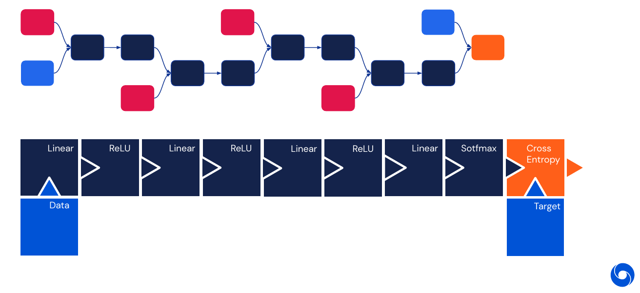
It is helpful to see neural networks as computational graphs on which we perform operations. Light blue nodes are data, input and target. Red blocks are parameters or weights which influence the operation in dark blue nodes. Note that not every operation node has parameters, this is only the case for linear layers in this example. Generally we pass the data from left to right (forward pass) and the gradients from right to left (backward pass).

Later levels in the network perform higher level tasks, such as line/corner detection compared to shape/object detection.

03 - Learning - 52:27

A quick recap on linear algebra (I would rather say calculus). The gradient of a function

\[\begin{align} f &: \mathbb{R}^n \longrightarrow \mathbb{R} \\ y &= f(\mathbf{x}) \end{align}\]

is

\[\frac{\partial y}{ \partial \mathbf{x}} = \nabla_{\mathbf{x}} f(\mathbf{x}) = \bigg[\frac{\partial f}{ \partial \mathbf{x}_1}, \dotsc, \frac{\partial f}{ \partial \mathbf{x}_2}\bigg]\]

The Jacobian of a function

\[\begin{align} f &: \mathbb{R}^d \longrightarrow \mathbb{R}^k \\ \mathbf{y} &= f(\mathbf{x}) \end{align}\]

is

\[\frac{\partial \mathbf{y}}{ \partial \mathbf{x}} = J_{\mathbf{x}} f(\mathbf{x}) = \begin{pmatrix} \frac{\partial f_1}{ \partial \mathbf{x}_1} & \dotsc & \frac{\partial f_1}{ \partial \mathbf{x}_d} \\ \vdots & \ddots & \vdots \\ \frac{\partial f_k}{ \partial \mathbf{x}_1} & \dotsc & \frac{\partial f_k}{ \partial \mathbf{x}_d} \\ \end{pmatrix}\]

Gradient descent is then for a sequence of parameters \(\mathbf{\theta_t}, t \in \mathbb{N}\):

\[\mathbf{\theta_{t+1}} := \mathbf{\theta_t} - \alpha_t \nabla_{\mathbf{\theta}} L(\mathbf{\theta_t})\]

where \(\alpha_t\) is the learning rate at time \(t\). Choosing a correct learning rate is crucial. In the case of non-convex “smooth enough” functions this converges to a local optimum. For each in the computational graph we pass the input in the forward pass and the gradient with respect to the loss function in the backward pass.

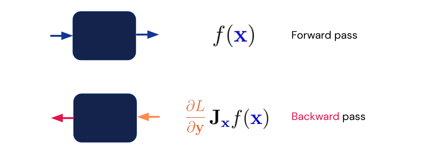
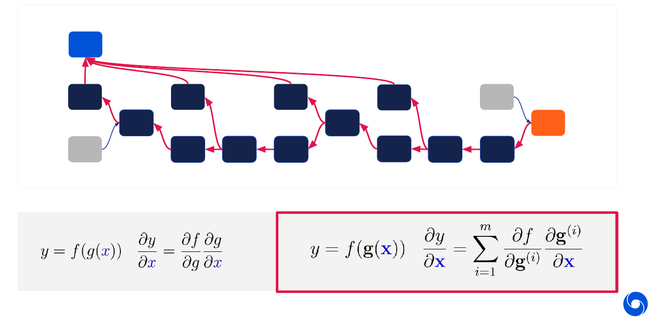
The whole optimization process is built on a few basic principles. The first one is automatic differentiation, for most loss functions and layers we have programs such as TensorFlow or PyTorch which are able to automatically differentiate the common loss functions and layers. No manual gradient calculation is required. There are two fundamental tools which are applied throughout the graph. The first is the chain rule visualized in the image below and written in its basic form on the box on the lower left.

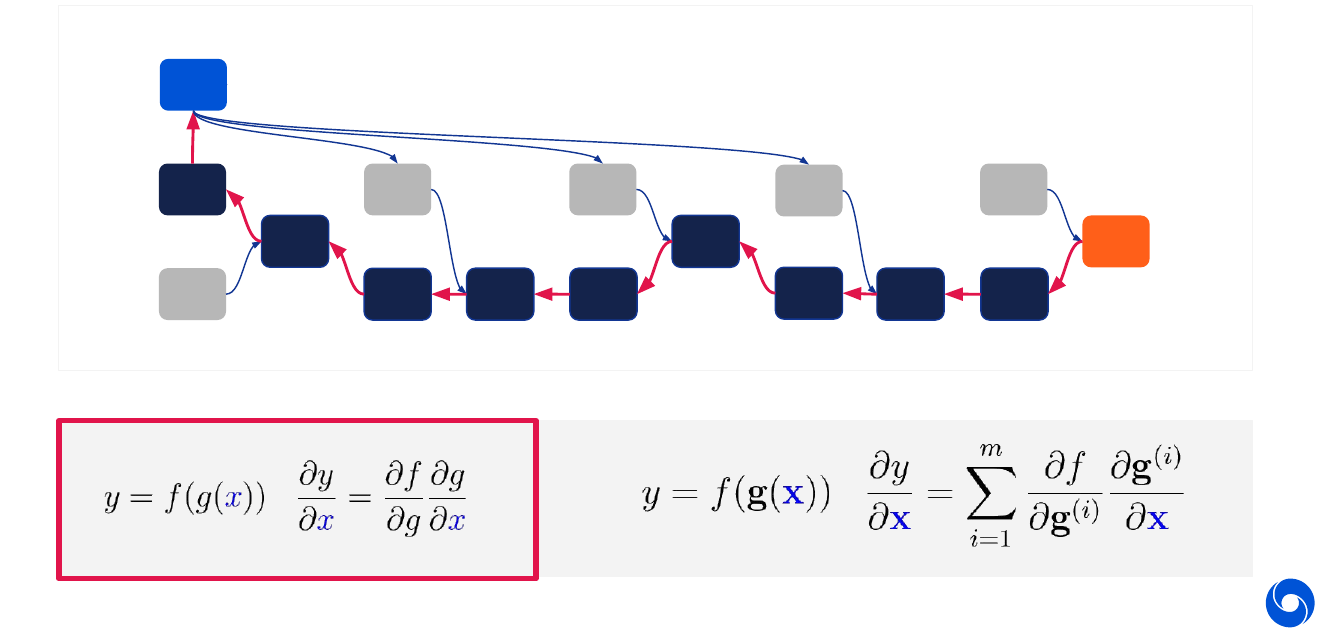
The other tool is back-propagation visualized in the graph below. It allows us to calculate the partial derivatives efficiently for each node (linear in the number of nodes).

A basic example of how the forward and backward pass work for a linear layer is illustrated below. Note that the derivative is taken with respect to the two parameters \(W\) and \(b\) as well as the input \(x\).

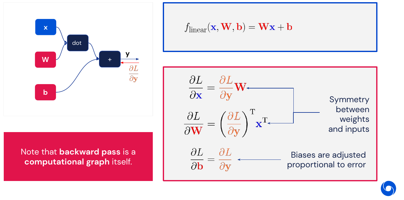
The same can be done for other parts of the network, for more details check the presentation. Note that for numerical stability the cross-entropy of logits is usually done in a single operation.

Remark: For more details on the forward and backward pass of these basic building blocks see my blog post on building a neural network from scratch

04 - Pieces of the Puzzle - 1:08:20

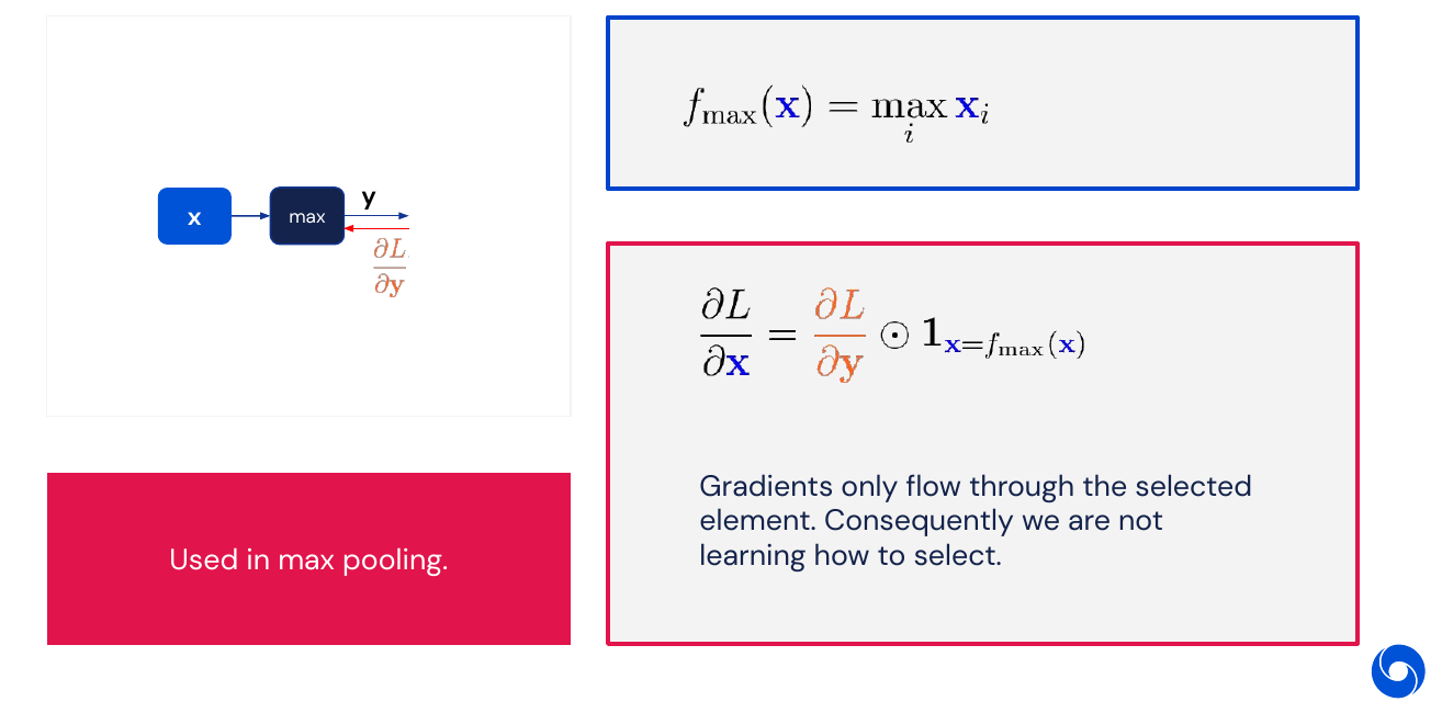
Other frequent operations used in neural networks are the max operation, where gradients only flow through the element which is maximal. This is a part of max pooling. No parameters can be learned

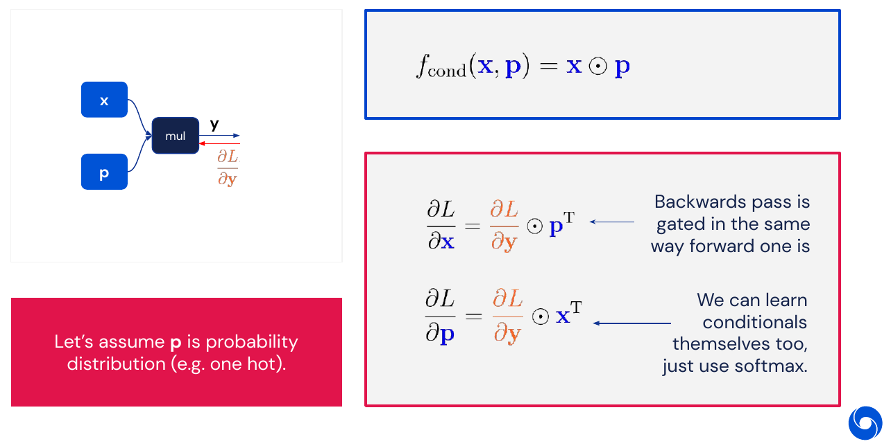
Another way of choosing which elements to pass forward is to do element wise multiplication such as in an attention layer (see lecture 8). Here it is possible to learn the probability distribution (using softmax).

05 - Practical Issues - 1:10:44

A classical problem in ML is over-fitting, our model has too many parameters and learns the training data set too precisely. Hence it will perform poorly on the test set, it does not generalize. There are a couple of techniques which can help mitigate or avoid those cases for neural networks:

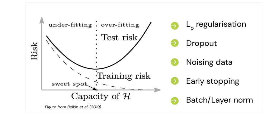
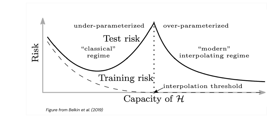
The above are classical results from statistics and Statistical Learning Theory, however this isn’t always true for neural networks. There are cases where the model initially becomes worse, before it becomes better again when we increase parameters (double descent). These are very recent results from 2019. What this tells us is that model complexity is not as simple as the number of parameters they have. Even if bigger models don’t necessarily over-fit anymore, they can still benefit from regularization techniques.

Training, diagnosing and debugging neural networks is not always easy. Often they fail silently, unlike classical programs a bug is not obvious and won’t make your program crash instantly. Here are some pointers to verify the correctness:

• Be careful with initialization
• Always over-fit on a small sample first (can highly recommend this, the simplest test to see if your basic setup works)
• Monitor training loss
• Monitor weight norms and NaNs (in my experience a NaN loss or accuracy is the closest you get to an obvious bug)
• Add shape asserts (to detect when your NN framework broadcasts a parameter into a different shape than you expect)
• Start with Adam (optimizer)
• Change one thing at a time (Something I can recommend highly from experience, otherwise it is almost impossible to attribute changes in accuracy to changes in code/data. In papers this is called ablation studies)

More detailed information can be found in Karpathy’s blog post.

06 - Bonus: Multiplicative Interactions - 1:19:48

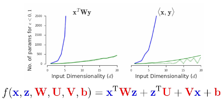
What can Multi Layer Perceptrons (MLPs) not do?

\[f(x,y) = \langle x,y \rangle\]

They can not represent multiplication. As the graphs below show, the number of parameters required to approximate multiplicative interaction grows exponentially with the number of input dimension. Being able to approximate something is not the same as being able to represent it. Approximation can be highly inefficient.

Closing words:

“If you want to do research in fundamental building blocks of Neural Networks, do not seek to marginally improve the way they behave by finding a new activation function. Ask yourself what current modules cannot represent or guarantee right now, and propose a module that can.”

Remark: This is something I can wholeheartedly agree with, too many of todays papers are happy to show an increase in 0.5% in accuracy in some benchmark, by doing a minor tweak.

My Highlights

• Approximation is not the same as representation
• XOR example with two layers
• Universal Approximation Theorem
• ReLu can be seen as folding space on top of each other (paper)
• Deep Double Descent and over-parametrization in neural networks
• MLPs and multiplicative operations (paper, follow up read)

Episode 3 - Convolutional Neural Networks for Image Recognition

01 - Background - 1:30

What is an image? An image is a 2D grid of pixels, but neural network expect a vector of numbers as an input. So how can we transform it? One way is by flattening the grid to a vector, simply attaching each row at the end of the previous one. One issue with this is, if we shift the input in the original space by some pixels, it will produce a completely different input. The case is illustrated below.

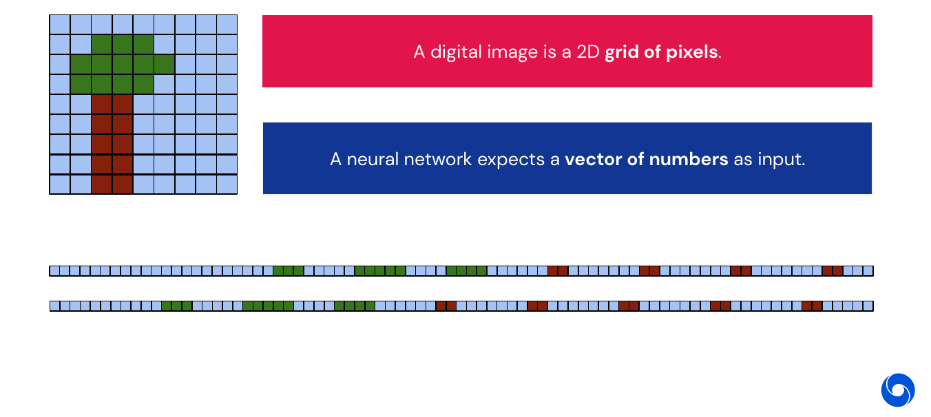
Moreover we would also want to make the network take into account the grid structure of an image. We can summarize this in two key features:

• Locality: nearby pixels are strongly correlated
• Translation invariance: patterns can occur anywhere in the image

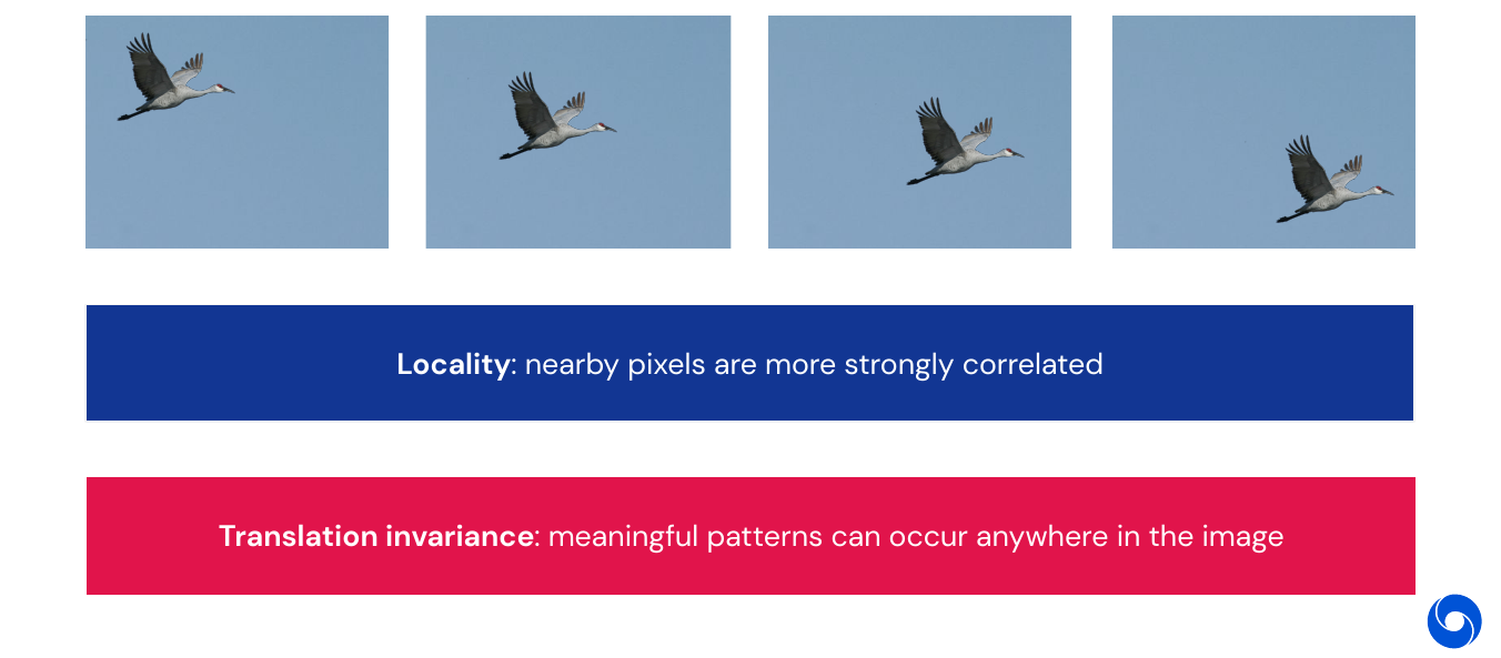
The above is true for images but also for other modalities, for example sounds can occur at any time in a signal. This is translation invariance in time. And in textual data, words can occur in any place. In graph structures, molecules can exhibit patterns anywhere. How can we put these properties into a network and take advantage of topological structure? By using the two following properties

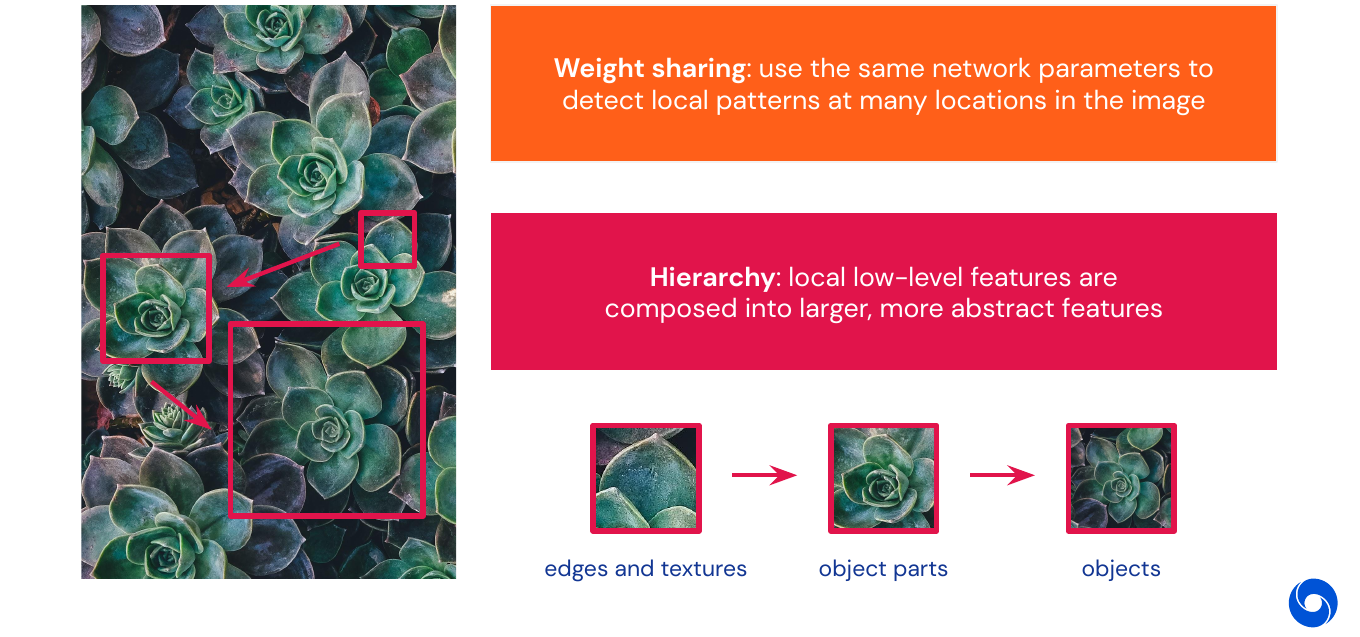
• Weight sharing: use the same parameters to detect the same patterns all over the image
• Hierarchy: low-level features are composed, model can be stacked to detect these

02 - Building Blocks - 19:46

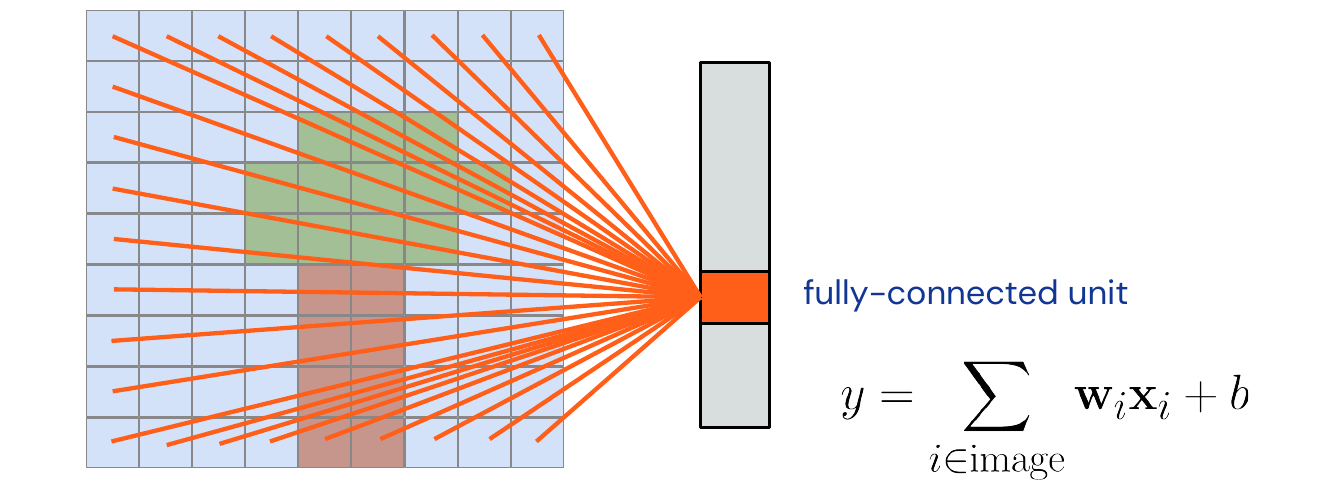
What we want to do is going from a fully connected operator below to a locally connected one. Note that the image does not really display a fully connected layer, there are all connections missing which do not occur at the border of the image (keeps the graphic readable).

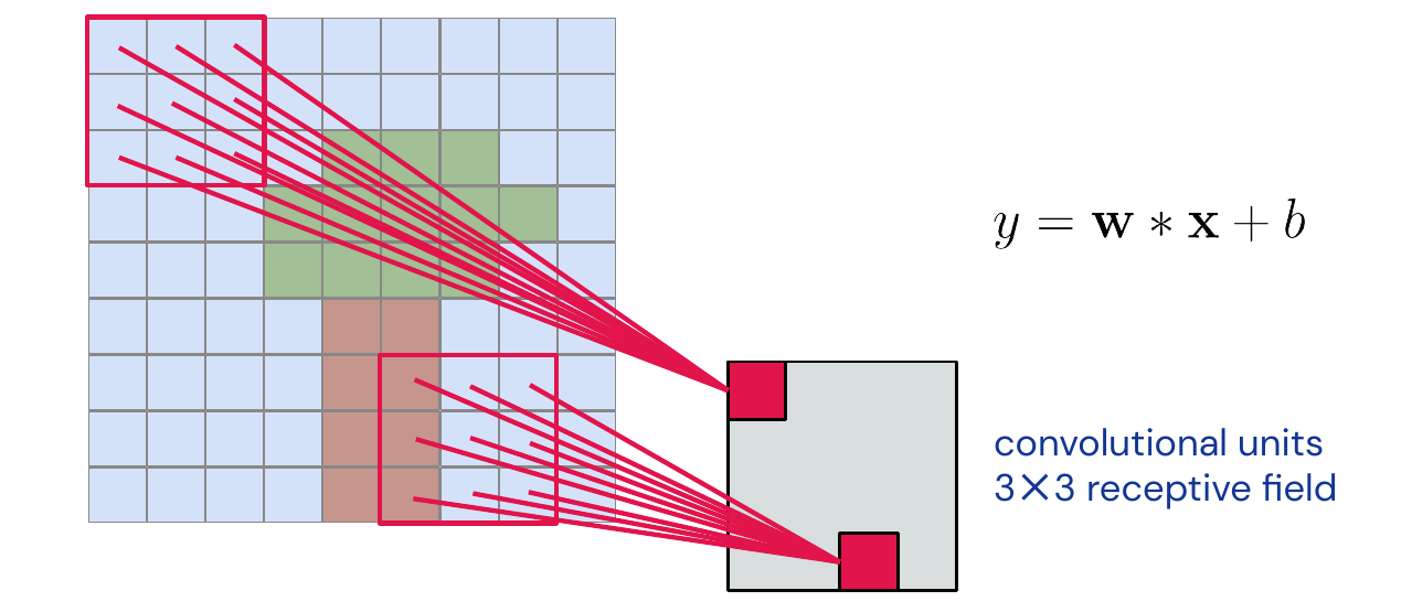
The example below shows how we force the network to be locally connected and share the same weights over all the image: a 3x3 convolution. The operation becomes equivariant to translation. In the context of neural networks we often call the weights kernel or filter. This kernel slides over the whole image and produces a feature map. For each pixel in the feature, map we call the input which goes into the calculation for that pixel the receptive field.

In a real world application, we will always have more than one filter. Each of them will go over the input and produce a feature map, these feature maps are often called channels.

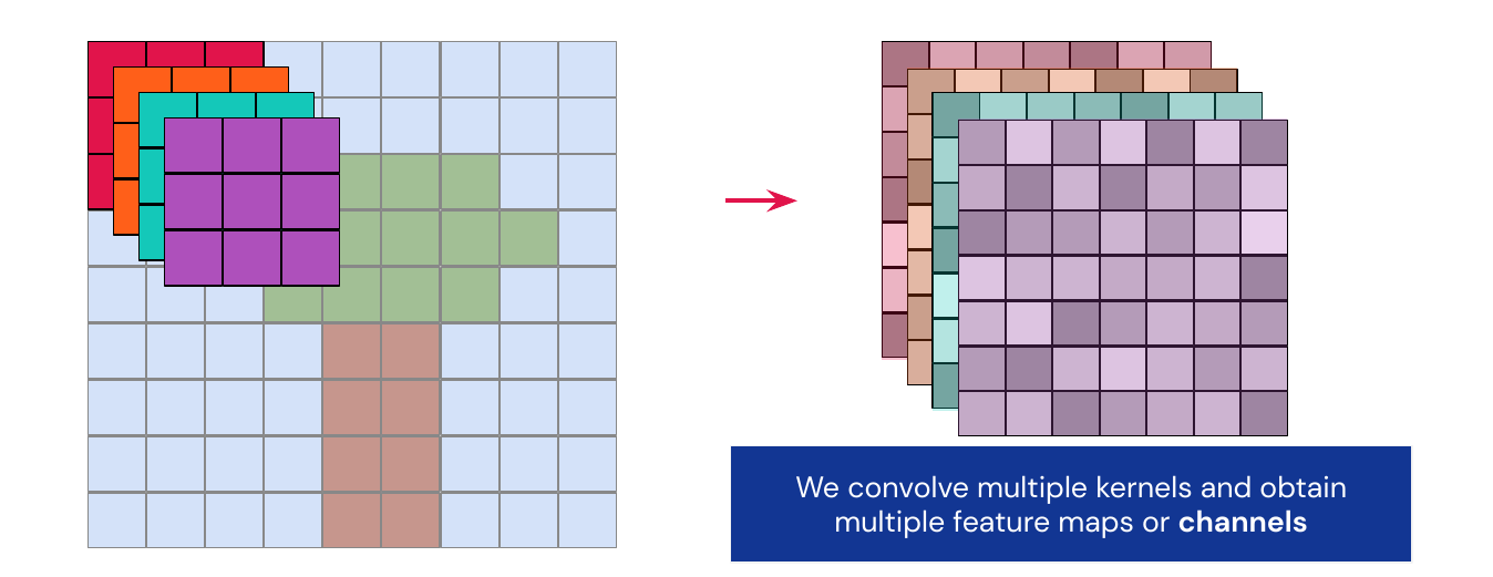
Convolutions are essentially filter operations with learned weights. There are many variants of the convolution operation:

• Valid convolution: no padding, slightly smaller output
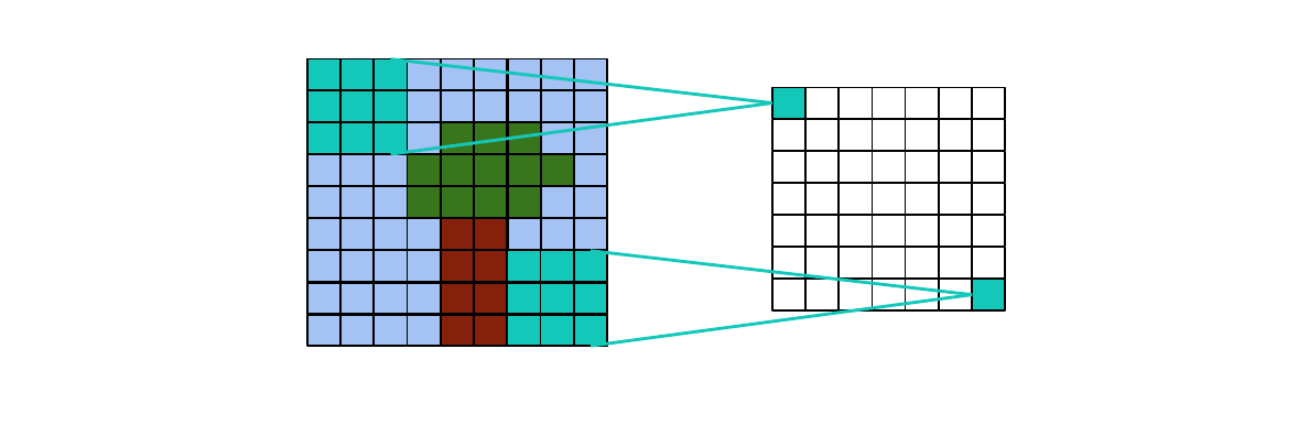
• Full convolution: padding so that only one pixel overlaps in minimum, larger output than input
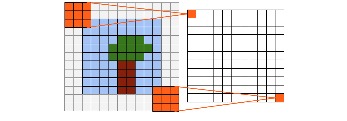
• Same convolution: padding so that output has same size as input, works better for odd kernel size
• Strided convolution: step size > 1, makes the output resolution by at least 2x smaller
• Dilated convolution: kernel is spread out, increases receptive field, step size > 1 inside kernel. Can be implemented efficiently
• Depthwise convolution: Normally each input channel is connected to each output channel, here every input channel is connected to only one output channel
• Pooling: compute mean or max over small windows

03 - Convolutional Neural Networks - 35:32

A basic convolutional neural network has the structure of the graph in the image below. We stack blocks of convolutions, non-linearity and pooling together and repeat them as many times as possible. In the end there are some blocks consisting of fully-connected and non-linearity layers. This structure is typical for networks used for classification. Note that we will not use explicit blocks for weights and loss functions anymore.

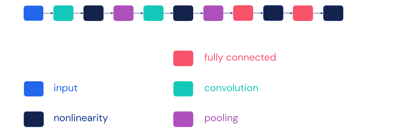
04 - Going Deeper: Case Studies - 38:10

Here we are going to see the most important evolutionary steps in neural network for images. They will address some of the key challenges of deep networks: computational complexity and optimization. Some of the techniques that can help are: initialization, sophisticated optimizers, normalizations layers and network design. Lets start simple with the example from the previous image:

• LeNet-5 (1998): Has 5 layers, sigmoid (used for handwritten digit recognition)

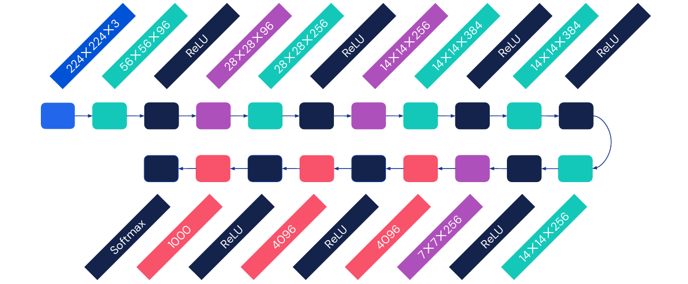
• AlexNet (2012): Has 8 layers, ReLU, start with a 11x11 kernel, not every convolution needs to be followed by pooling

• VGGNet (2014): up to 19 layers, use same convolutional layers to avoid resolution reduction. Only uses 3x3 kernels and stacks them instead of larger kernels.

  Stacking increases the receptive fields with fewer parameters and more flexibility

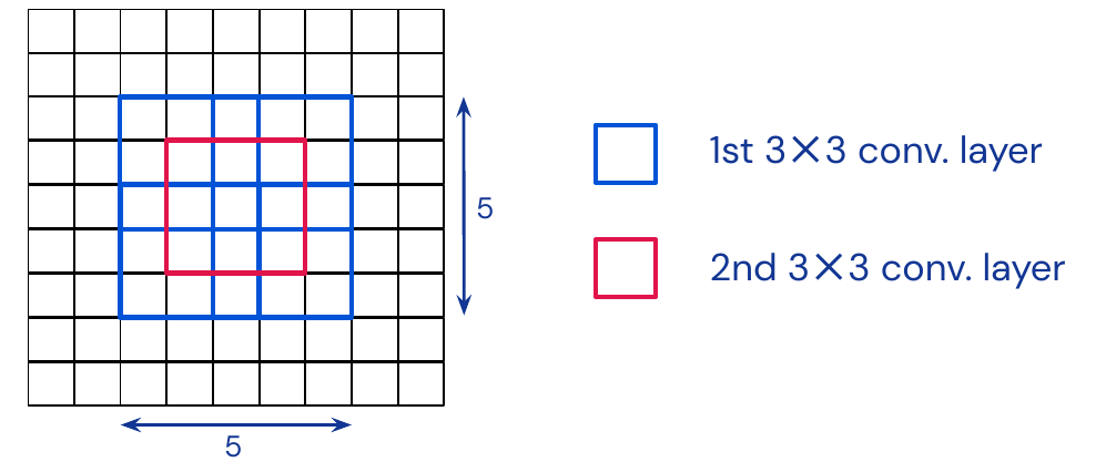
  Interestingly the error plateaus at 16 layers, training a network with 19 layers was worse. This is because deeper networks are harder to optimize. There are two main innovations which made deeper networks more trainable:

• Batch Normalization: Normalize each input pixel over the batch dimension by subtracting the mean \(\mu\) and dividing by the standard deviation \(\sigma\). Multiply the result by \(\gamma\) and add \(\beta\), both are learnable parameters. This simple idea reduces sensitivity to initialization and acts as a regularizer. It makes networks more robust to different learning rates and introduces stochasticity (because \(\mu\) and \(\sigma\) have to be re-estimated for each batch). However at test time this introduces dependency on other images in a batch. What we generally do is to freeze those values for tests, this can be a source for a lot of bugs.

• Residual connections, introduced in ResNet (2015): The ResNet architecture can be up to 150 layers deep. It is able to do that because it introduces residual connections, which make training deeper networks simpler by letting the network ‘choose’ which layers it needs. In the simplest case the network can be an identity function.

  Generally the first convolution acts as a bottleneck block, applying a 1x1 convolution to reduce channels. Then a 3x3 convolution can be applied on fewer channels, allowing for lower computational costs and fewer parameters. Finally a last 1x1 convolution restores the original number of channels. Interestingly this setup allows the ResNet-152 to be computationally cheaper than than VGG network. The version 2 avoids nonlinearities in residual pathways.

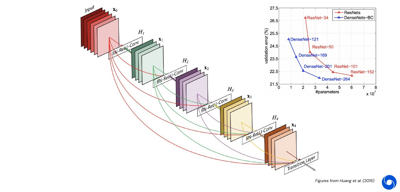
• DenseNet (2016): connections to all previous layers, not only one

• AmoebaNet (2018): One of the first architectures not designed by a man but but by an algorithm. This is called neural architecture search, here an evolutionary search algorithm was used. The network is basically an acyclic graph composed of predefined layers.

• Other ways to reduce complexity of networks:
  • Depthwise convolutions
  • Separable convolutions
  • Inverted bottlenecks (MobileNetV2, MNasNet, EfficientNet)

05 - Advanced Topics - 1:09:40

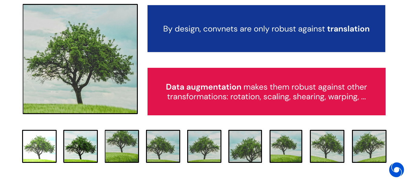
So far we have seen networks being robust to translation. Using data augmentation, we can make them robust against other transformations: rotation, scaling, shearing, warping and many more.

We can visualize what a convolutional network learns, by maximizing one activation using gradient ascent. Even with respect to a specific output neuron (class).

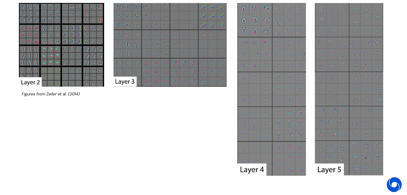
For more details and explanations, read the article on distill.pub, Other topics:

• Pre-training and fine-tuning
• Group equivariant convnets: invariance to e.g. rotation and scale
• Recurrence and attention (these are discussed in later lectures)

06 - Beyond Image Recognition - 1:16:32

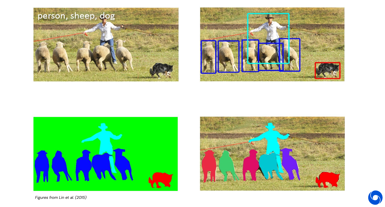
Other tasks beyond classification are: Object detection (top right), semantic segmentation (bottom left), instance segmentation (bottom right). We will see more of them in future lectures.

My Highlights

• BatchNorm introduces stochasticity

Episode 4 - Advanced models for Computer Vision

Holy grail: Human level scene understanding.

01 - Supervised image classification - Tasks beyond classification - 5:20

Task 1 - Object Detection

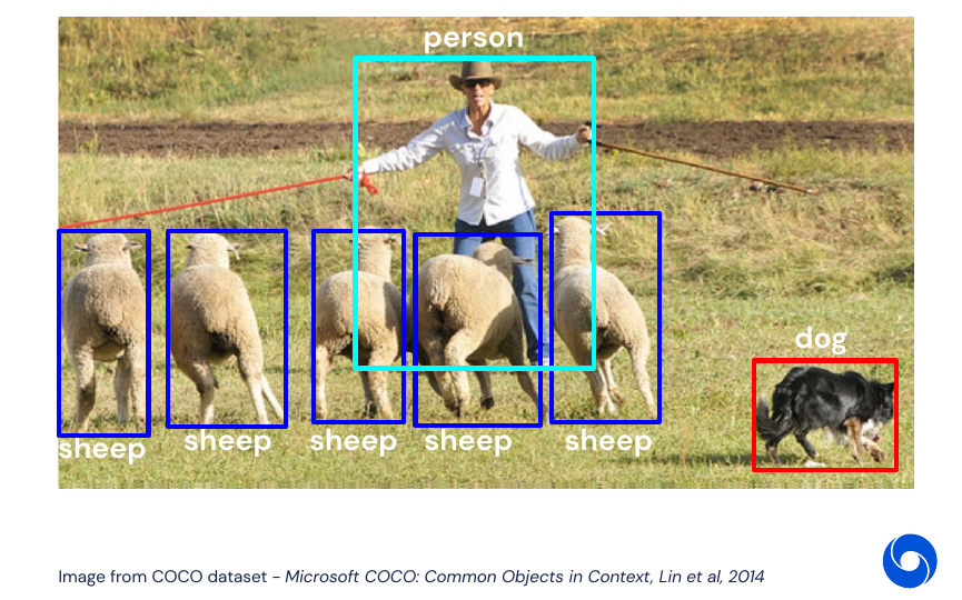
The input are again images. The output is a class label which is one hot encoded and a bounding box with \((x_c, y_c, h, w)\) for every object in the scene. The data is not ordered and we do regression on coordinates. Generally minimize quadratic loss for regression task \(l(x,y) = \| x-y\|^2_2\).

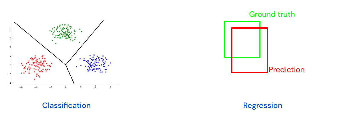
How to deal with multiple targets? Redefine problem, first do classification and then regression by discretization of output the values in one hot encoded labels.

Case studies:

Faster R-CNN, Two-Stage Detector

When we redefine the problem we need to set up anchor points over the image, these are centers of candidate bounding boxes and correspond to the \((x_c, y_c, h, w)\) part of the problem.

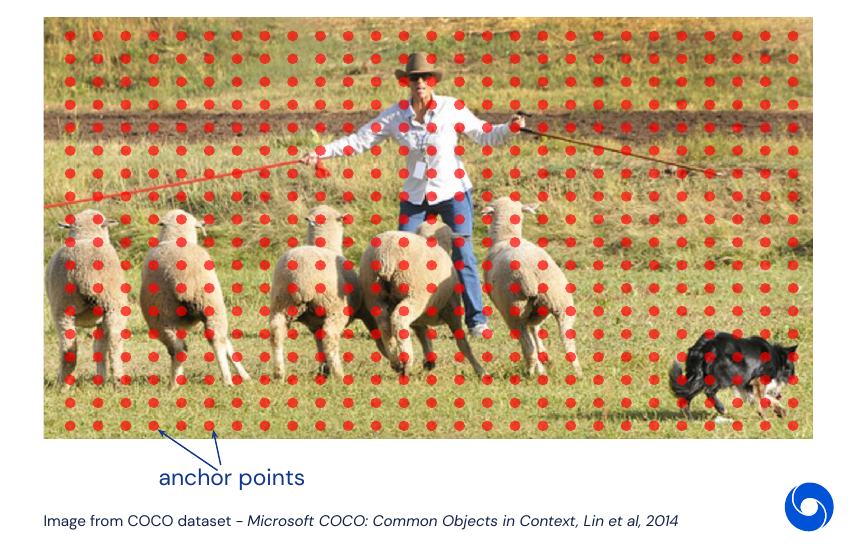
For each of these anchor points we add multiple candidate bounding boxes. They have different scales and ratios for height and width \((h, w)\). For each combination of anchor point and bounding box an objectness score will be predicted. In the end they are sorted and the top K will be kept.

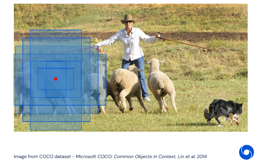
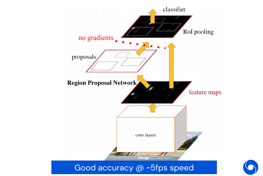
These top K predictions are then passed through another small MLP which will refine them further by performing regression. This is a so called two-stage detector as a non-differentiable step is involved. This means we have to train the system in two parts, one which predicts objectness and and the second which performs the regression on the result of the first one. This system achieves good accuracy at a speed of approximately 5 frames per second. There exist versions which involve only differential operations, as for example in Spatial Transformer Networks.

RetinaNet - One-Stage Detector

One way of solving the two stage problem is to predict classes and coordinates of bounding boxes straight away. The RetinaNet architecture uses a feature pyramid network to combine semantic with spatial information for more accurate predictions. A basic ResNet architecture extracts features which are then up-sampled back to a higher resolution and enriched with spatial information from earlier stages of the network using skip connections. For each level of the pyramid layer K classes and A anchor boxes are predicted. A parallel network will predict four regression coordinates for each anchor box.

However this construction will not train out of the box with a standard loss such as cross-entropy. The problem is the large class imbalance, out of thousands of bounding boxes almost all of them will be background. Even if they are classified with high confidence, their sheer number will overwhelm the signal generated by the rare useful examples. Even if we correctly assign a high probability (i.e. > 0.6) to the background class, the loss value will still be significantly larger than zero.

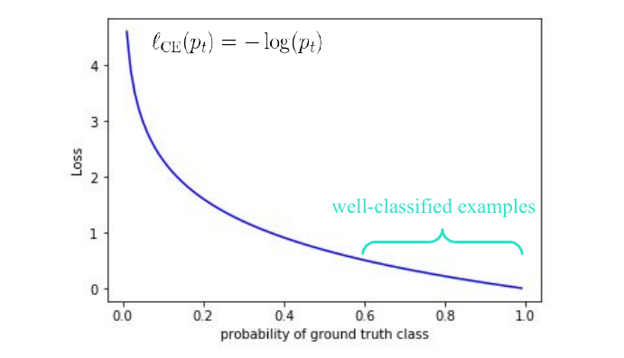
Faster R-CNN pruned most of these easy negatives in the first stage during the sorting. One-stage detectors solved the problem by employing hard negative mining procedure:

1. Get set of positive examples
2. Get a random subset of negative examples (as the full set of negatives is too big)
3. Train detector
4. Test on unseen images
5. Identify false positive examples (hard negatives) and add them to the training set
6. Repeat from step 3

However one of the main contributions of RetinaNet was the introduction of focal-loss:

\[l_{CE}(p_t) = -(1-p_t)^{\gamma}\log(p_t)\]

Where \(\gamma\) is a hyper-parameter, \(\gamma=0\) corresponds to a classical cross-entropy loss. The introduction of this additional factor of \((1-p_t)^{\gamma}\) reduces the loss of high confidence examples enough to make training stable without additional procedures such as hard negative mining.

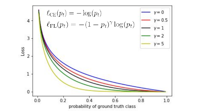
This development lead to new state of the art results at 8 frames per second.

Task 2 - Semantic Segmentation

Semantic Segmentation is the task of assigning each pixel to a class. The problem here is to generate an output at the same resolution as the input. All the examples we have seen so far have sparse output.

The spatial resolution loss is mostly caused by the pooling layers, which create a larger receptive field at the expense of spatial information. Hence we need a reverse operation, some examples which do ‘unpooling’ operations are: unpooling, upsampling, deconvolutions.

U-Net

The U-Net architecture follows an encoder-decoder model, with skip connections to preserve high frequency details. A pixel-wise cross-entropy loss is applied to the output.

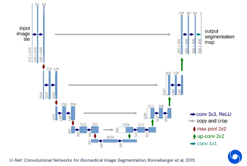
The skip connections are similar to the residual blocks in the ResNet architecture, they help back-propagating the gradients, and make the network easier to optimize. The architecture is also closely related to what we saw the previously in RetinaNet, where the architecture was described as feature pyramid architecture, they both follow an U shape.

Task 3 - Instance Segmentation

If we combine object detection with semantic segmentation, then we get instance segmentation. It allows us to separate overlapping classes, such as multiple sheep in the same image below. The general setup for instance segmentation is very similar to object detection, individual objects are predicted with a bounding box, but then an additional semantic segmentation head is applied to get more precise contours. The model generally used for instance segmentation is very similar to Faster R-CNN and is called Mask R-CNN.

Metrics and Benchmarks

Classification was easy: Accuracy as percentage of predictions. Sometimes we also use metrics which count a prediction as correct when it is in the top-5.

Object detection and segmentation: Intersection over Union (non-differentiable, so it’s only for evaluation).

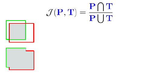
Pixel wise accuracy would be foolish to use. Not recommended in general to use different measures between training and testing. (IoU not differentiable because of max operations)

Remark: Here some more details would have been nice. While for semantic segmentation, IoU or rather mIoU (mean Intersection over Union) is frequently used, in object detection mAP (mean average precision) is more common. While it is also based on IoU, it adds another layer of complexity on top.

Some common benchmark sets used to evaluate those tasks: cityscapes for semantic segmentation and COCO for instance segmentation.

Tricks of the Trade

Transfer learning. Reuse knowledge learned on one task on another one. Formally: Let

\[\mathcal{D} = \lbrace \mathcal{X}, P(X) \rbrace, X = \lbrace x_1, \dotsc, x_n \rbrace \in \mathcal{X}\]

be a domain and

\[\mathcal{T} = \lbrace \mathcal{Y}, f( \cdot ) \rbrace, f(x_i) = y_i, y_i \in \mathcal{Y}\]

a task defined on this domain. Given a source domain task \(\begin{pmatrix} \mathcal{X}_S \\ \mathcal{T}_S \end{pmatrix}\) and a target domain task \(\begin{pmatrix} \mathcal{X}_T \\ \mathcal{T}_T \end{pmatrix}\), re-use what was learned by \(f_S : \mathcal{X}_S \longrightarrow \mathcal{T}_S\) in \(f_T : \mathcal{X}_T \longrightarrow \mathcal{T}_T\).

Remark: This definition seems to be very close to what can be found on Wikipedia.

The intuition is that features are shared across tasks and dataset. No need to start from scratch all the time. Reuse knowledge across tasks or across data.

• Transfer learning across different tasks: Mostly remove the last layers and add new layers to adapt to the new task. See Taskonomy paper, for an overview of different tasks and how they are related.
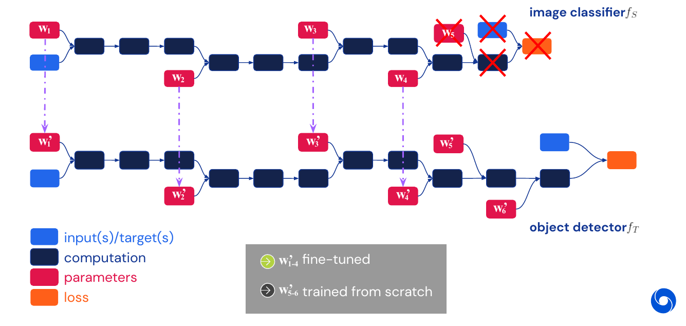
• Transfer learning across different domains: Train in simulation, test in the real world. Use tricks to adapt to target domain (for example domain randomization and hard negative mining to identify the most useful augmentations)

02 - Supervised Image Classification - Beyond Single Image Input - 50:26

Experiments with people who recovered from blindness after a surgery allowed for insights to which tasks are hard. They were asked to recover objects from a scene. They had trouble identifying objects in some scenarios. However if you show them the same type of images, but with moving images then they do much better. Motion really helps with object recognition when learning to see. Conclusion: should use videos for training object recognition.

Input - Pairs of images

What is optical flow estimation? Input are two images, for each pixel in image one \(I_1\), we would like to know where it did end up in image two \(I_2\). The output is a map of pixel wise displacement information, for horizontal and vertical displacement.

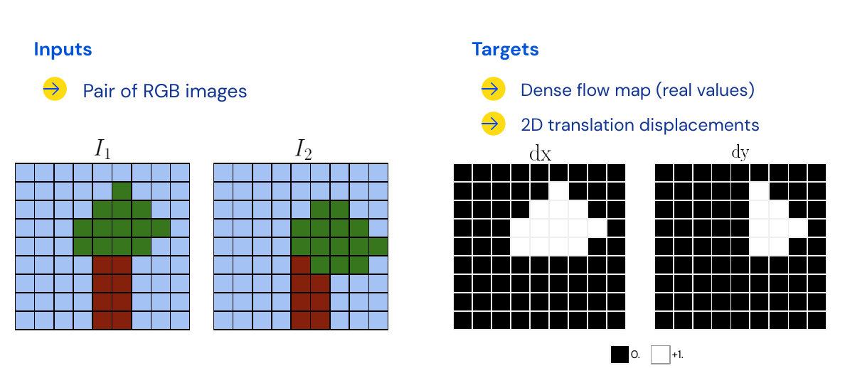
Case Study: FlowNet

Encoder-Decoder architecture like U-Net, fully supervised with euclidean distance loss. Invented Flying chairs dataset with sim to real to learn about motion. Essence is that pixels that move together belong to the same object.

Input - Videos

Base case: use semantic segmentation video and apply it frame wise (but don’t use temporal information), this leads to flickering in a video. We could use 3D convolutions by stacking 2D frames to get volumes, kernels are 3D objects. In 3D convolutions the kernel moves in both space and time to create spatio-temporal feature maps (we can re-use strided, dilated, padded properties).

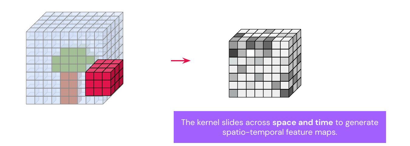
3D convolutions are non-causal, because you take into account frames from the future (times \(t-1, t, t+1\)), which is fine for off-line processing, but when applying it in real time we have to use masked 3D convolutions.

These networks can do action recognition: using video as input while the prediction target is an action label which is one-hot encoded.

Case Study: SlowFast

SlowFast is a two branch model which takes inspiration from the human visual system, which has also two streams:

• Hight frame rate branch: Less features, tracks high frequency changes.
• Low frame rate branch: More features, abstract information stays the same over longer time frame.

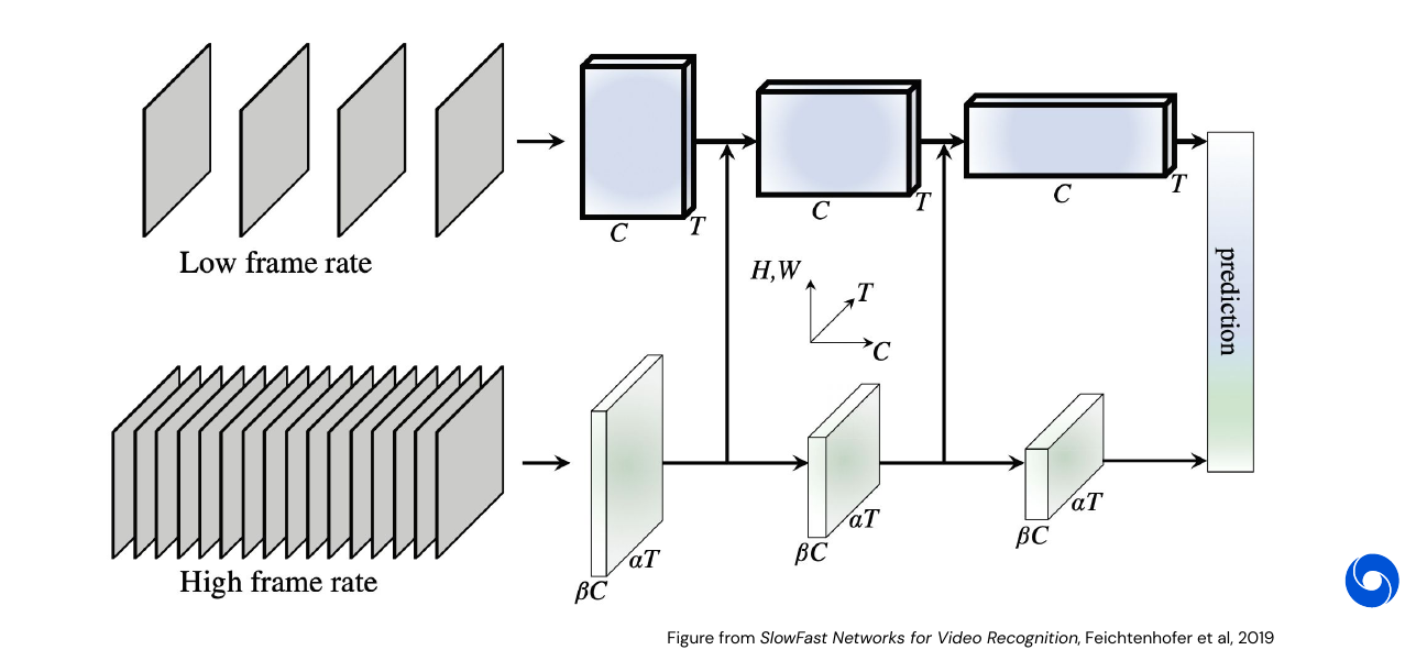
Transfer learning can be used by inflating 2D image filters to 3D filters by replicating them along the time dimension.

Challenges in Video Processing

It is difficult to obtain labels, models have large memory requirements, high latency, and high energy consumption. Basically we need too much compute for it to be broadly applicable. Ongoing area of research of how to improve that by using parallelism and exploit redundancies in the visual data. One idea is to train a model to blink, (humans do it more often than necessary to clean the eye, it might be used to reduce cognitive load).

03 - Supervised Image Classification - Beyond Strong Supervision - 1:20:23

Labeling is tedious and a research topic on itself. Humans can only label key-frames and methods will propagate labels. Example: PolygonRNN.

Self-Supervision - Metric Learning

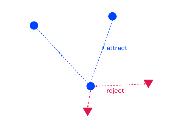
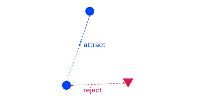
Standard losses such as cross-entropy and mean square error learn a mapping between input and output. Metric learning learns to predict distances between inputs in an embedding to give similarity measure between data. Create clusters with same person, for unseen data use nearest neighbor.

Used for learning self-supervised representations, information retrieval and low-shot face recognition.

Contrastive Loss

Also called margin loss, data is triplets \((r_0, r_1, y)\) where \(y=1\) if \(r_0\) and \(r_1\) are the same person and \(y=0\) otherwise. The loss function is then

\[l(r_0, r_1, y) = y d(r_0, r_1)^2 + (1-y)\big(\max(0, m-d(r_0, r_1))\big)^2\]

where \(d(\cdot, \cdot)\) is the Euclidean distance. We use the margin \(m\) to cap the maximal distance, however it is hard to choose a value for \(m\). All classes will be clustered in a ball of radius \(m\), which can be unstable.

Triplet Loss

Use triplets \((r_a, r_p, r_n)\) where \((r_a, r_p)\) are similar and \((r_a, r_n)\) are dissimilar (\(p\) for positive and \(n\) for negative example). The loss function is then:

\[l(r_a, r_p, r_n) = \max(0, m+d(r_a, r_p)^2 - d(r_a, r_n)^2)\]

This works better than the contrastive loss because relative distances are more meaningful than a fixed margin. However one needs hard negative mining to select informative triplets for training.

State-Of-The-Art

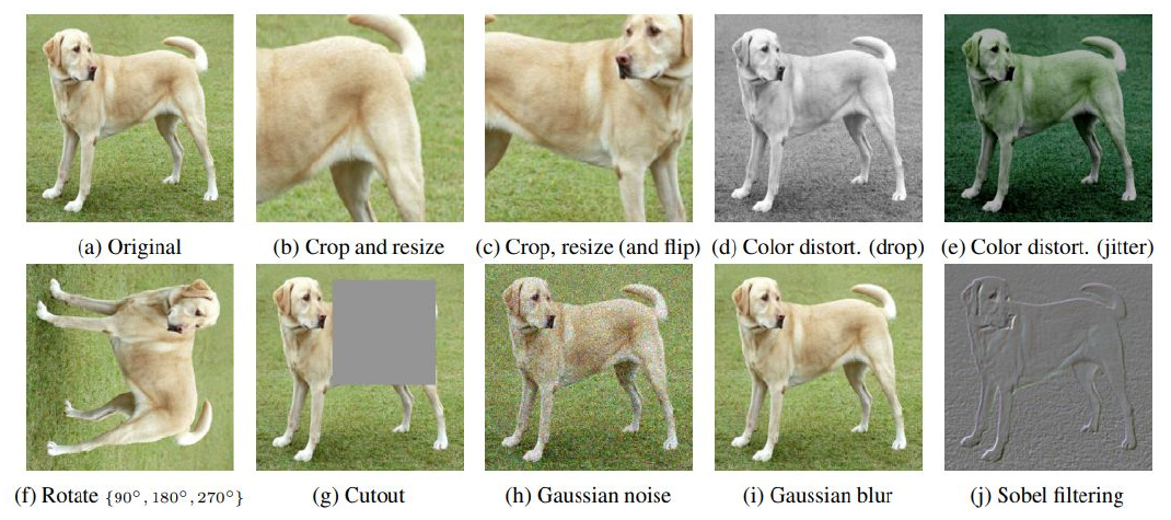
The current state of the art uses the same data, but different augmentations. Especially compositions of data augmentations are important, results are comparable to a supervised ResNet-50 (although with more parameters).

04 - Open Questions - 1:30:16

Is vision solved? What does it mean to solve vision? We need the right benchmarks.

How to scale systems up? Need a system that can do all the tasks at once, more common sense. Different kind of hardware.

What are good visual representations for action? Key-points could help.

Conclusion

Need to rethink vision models from the perspective of moving pictures with end goal in mind.

My Highlights

• Finally a good explanation of the difference between two-stage and one-stage detection (try googling the difference),
• Connection between object detection and semantic segmentation via U-Net structure.
• Motion helps when learning to see
• Non-causality of 3D convolutions

Episode 5 - Optimization for Machine Learning

01 - Introduction and Motivation - 0:42

Optimization algorithms enable models to learn from data by adapting parameters to minimize an objective function. This works by making small incremental changes to model parameters which each reduce the objective by a small amount. Examples are prediction errors in classification or negative rewards in reinforcement learning. We use the following notation:

• Parameters: \(\theta \in \mathbb{R}^n\), where \(n\) is the dimension.
• Real-valued objective function: \(h(\theta)\).
• Goal of opimization: \(\theta^* = \text{arg min}_{\theta} h(\theta)\).

An example of an objective function in the 1D space:

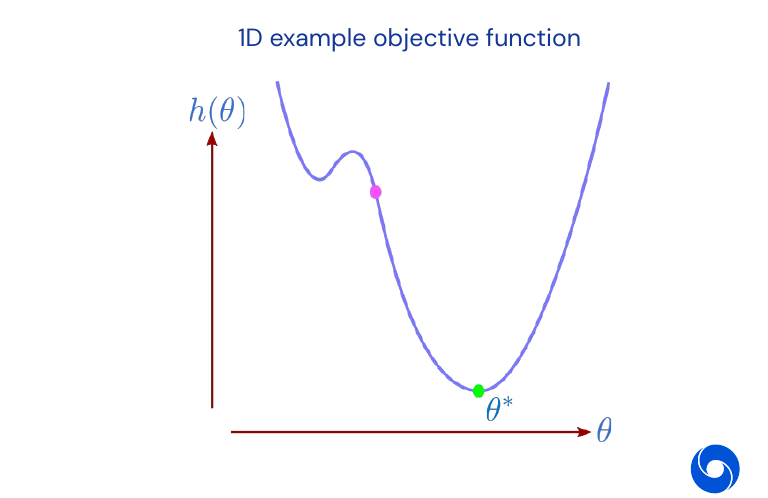
A standard neural network training objective is

\[h(\theta) = \frac{1}{m} \sum^m_{i=1} l(y_i, f(x_i, \theta))\]

where \(l(y, z)\) is a loss function measuring the disagreement between label \(y\) and prediction \(z\). And \(f(x, \theta)\) is a neural network function taking input \(x\) and outputting some prediction. Note that we are summing over \(m\) examples.

02 - Gradient Descent - 4:12

A basic gradient descent iteration is:

\[\theta_{k+1} = \theta_k - \alpha_k \nabla h(\theta_k)\]

where \(\alpha_k\) is the learning rate (also frequently called step size) and

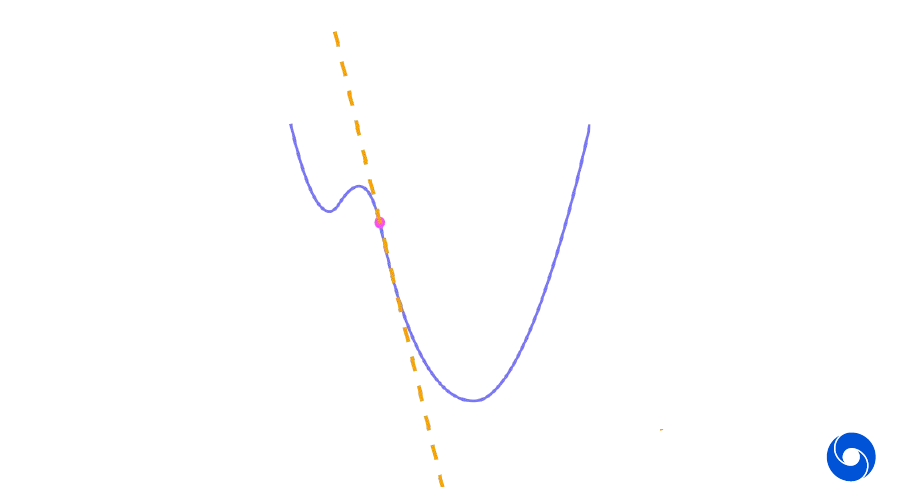
\[\nabla h(\theta) = \begin{pmatrix} \frac{\partial h(\theta)}{\partial \theta_1} \\ \frac{\partial h(\theta)}{\partial \theta_2} \\ \vdots \\ \frac{\partial h(\theta)}{\partial \theta_n}\end{pmatrix}\]

is the gradient, a \(n\)-dimensional vector. The intuition about gradient descent is it is the ‘steepest descent’. Gradient \(\nabla h(\theta)\) gives greatest reduction in \(h(\theta)\) per unit of change. There is the issue between high smoothness vs. low smoothness in the objective function, where low smoothness can make the optimization process much more challenging as shown in the example below.

Intuitively gradient descent is minimizing a local approximation. A first-order Taylor series approximation for \(h(\theta)\) around the current \(\theta\) is

\[h(\theta + d) \approx h(\theta) + \nabla h(\theta)^T d\]

Which is a reasonable approximation for small enough \(d\). A gradient update is computed by minimizing this within a sphere of radius \(r\):

\[-\alpha \nabla h(\theta) = \text{arg min}_{d: \| d \| \leq r} (h(\theta) + \nabla h(\theta)^T d) \qquad \text{where } r = \alpha \| \nabla h(\theta) \|\]

Remark: We can think of \(d\) as either direction vector or difference in the 1D case.

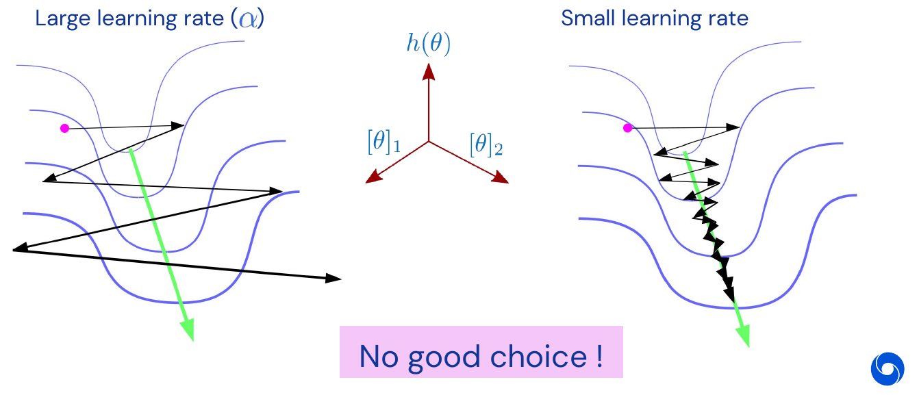
There are problems with gradient descent in multiple dimensions, as depicted in the narrow 2D valley in the image below. It is hard, if not impossible, to find a good learning rate. If it is too large it might leave the valley, if it is too small it might take too many steps to converge.

Convergence Theory

In convergence theory the following assumptions are made

• \(h(\theta)\) has Lipschitz continues derivatives:

  \[\| \nabla h(\theta) - \nabla h(\theta') \| \leq L \| \theta - \theta' \|\]

  This means gradient doesn’t change too much as we change parameters (upper bound on curvature)

• \(h(\theta)\) is strongly convex (perhaps only near a minimum):

  \[h(\theta + d) \geq h(\theta) + \nabla h(\theta)^T d + \frac{\mu}{2} \|d\|^2\]

  This means the function curves as least as much as the quadratic term (lower bound on curvature)

• For now: Gradients are computed exactly, i.e. not stochastic.

If the previous conditions apply and we take \(\alpha_k = \frac{2}{L+\mu}\) then

\[h(\theta_k) - h(\theta^*) \leq \frac{L}{2}\bigg(\frac{\kappa-1}{\kappa + 1}\bigg)^{2k} \| \theta_0 - \theta^*\|^2\]

where \(\kappa = \frac{L}{\mu}\). Remember that \(\theta^*\) is the value of \(\theta\) which minimizes the objective function \(h(\theta)\). We have that the number of iterations to achieve \(h(\theta_k) - h(\theta^*) \leq \epsilon\) is

\[k \in \mathcal{O}\bigg(\kappa \log\bigg(\frac{1}{\epsilon}\bigg)\bigg)\]

The important variable here is \(\kappa\), we prefer smaller values of \(\kappa\). It is the ratio between smallest curvature and highest curvature, often called condition number but is global here. This is similar to biggest eigenvalue in a Hessian divided by smallest one.

Remark: The smaller \(L\) the ‘better behaved’ the gradients of the function are, i.e. a small difference in \(\theta\) will not lead to a large move in \(\nabla h(\theta)\). This will lead to a smaller \(\kappa\) (as will a large \(\mu\) but this is less desirable as it is a lower bound on the smoothness). Why is a large \(\kappa\) bad? Because it will make the only term which depends on \(k\) be close to \(1 \approx \big(\frac{\kappa-1}{\kappa+1}\big)\) for \(\kappa \gg 1\) .

Is convergence theory useful in practice?

• It is often too pessimistic as it has to cover worst case examples
• Makes too strong assumptions (convexity), or too weak (real problems have more structure)
• It relies on crude measures such as condition numbers
• And most importantly: focused on asymptotic behavior, often in practice we stop long before that bound and there is no information about behavior in that part of the optimization process

Design/choice of an optimizer should always be more informed by practice than anything else, but theory can help to guide the way by building intuition. Be careful about anything ‘optimal’.

03 - Momentum Methods - 17:34

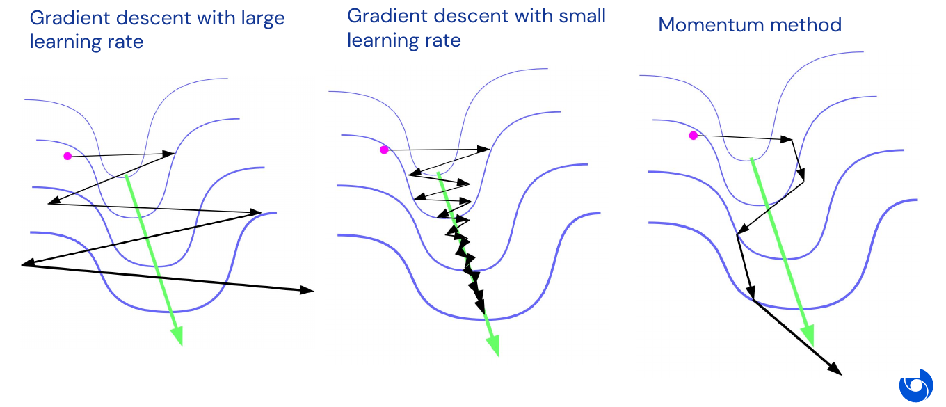
The main motivation for momentum methods is the tendency of gradient descent to flip back and forth, as in the narrow valley example. The key idea is to accelerate movement along directions that point consistently down-hill across many consecutive iterations (i.e. have low curvature). How would we do this? Use physics guidance like a ball rolling along the surface of the objective function (for a vivid illustration, checkout this youtube video). Two variants of momentum:

• Classical momentum:

  \[\begin{align} v_{k+1} &= \eta_k v_k - \nabla h(\theta_k) \qquad v_0=0 \\ \theta_{k+1} &= \theta_k + \alpha_k v_{k+1} \end{align}\]

  Where \(\alpha_k\) is the learning rate and \(\eta_k\) the momentum constant.

• Nesterov’s variant:
  \(\begin{align} v_{k+1} &= \eta_k v_k - \nabla h(\theta_k + \alpha_k \eta_k v_k) \qquad v_0=0 \\ \theta_{k+1} &= \theta_k + \alpha_k v_{k+1} \end{align}\)

In classical momentum we call \(v\) the velocity vector and \(\eta\) the friction. The Nesterov variant is more useful in theory, and also sometimes in practice. In the 2D valley example from above, the velocity keeps accumulating in the downward direction and never oscillates out of control.

Given the objective function \(h(\theta)\) satisfying the same technical conditions as before, and choosing \(\alpha_k\) and \(\eta_k\) carefully, Nesterov’s momentum method satisfies:

\[h(\theta_k) - h(\theta^*) \leq L \bigg(\frac{\sqrt{\kappa}-1}{\sqrt{\kappa}}\bigg)^{k} \| \theta_0 - \theta^*\|^2\]

for \(\kappa = \frac{L}{\mu}\). The number of iterations to achieve \(h(\theta_k) - h(\theta^*) \leq \epsilon\) is

\[k \in \mathcal{O}\bigg(\sqrt{\kappa} \log\bigg(\frac{1}{\epsilon}\bigg)\bigg)\]

For the upper bounds for the Nesterov momentum variant, the term now depends only on the square root of \(\kappa\), meaning the number of iterations is roughly the square root instead of linear. This makes bigger difference when \(\kappa\) is large, i.e. our function has high curvature.

In technical sense this is the best we can do for a first-order method. A first-order method is one where the updates are linear combinations of observed gradients, i.e.:

\[\theta_{k+1} - \theta_k = d \in \text{Span}\lbrace \nabla h(\theta_0), \nabla h(\theta_1), \dotsc, \nabla h(\theta_k) \rbrace\]

The following methods are of first-order:

• Gradient descent
• Momentum methods
• Conjugate gradients

What is not included is preconditioned gradient descent / second-order methods. Given the definition of first order method, we can get a lower bound which says we can not converge faster than \(\sqrt{\kappa}\). If we assume that the number of steps is greater than the dimension \(n\) (the number of parameters), and it usually is. Then, there is an example objective satisfying the previous conditions for which:

\[h(\theta_k) - h(\theta^*) \geq \frac{\mu}{2} \bigg(\frac{\sqrt{\kappa}-1}{\sqrt{\kappa} + 1}\bigg)^{2k} \| \theta_0 - \theta^*\|^2\]

with \(\kappa = \frac{L}{\mu}\). And the number of iterations to achieve \(h(\theta_k) - h(\theta^*) \leq \epsilon\)

\[k \in \mathcal{\Omega}\bigg(\sqrt{\kappa} \log\bigg(\frac{1}{\epsilon}\bigg)\bigg)\]

Remark: Remember from complexity theory that \(\Omega\) is the notation for the asymptotic lower bounds. So it will take at least \(\sqrt{\kappa} \log\big(\frac{1}{\epsilon}\big)\) iterations (up to some constant) to approximate the optimum up to a distance of \(\epsilon\).

We can compare all the bounds we have seen so far:

• (Worst-case) the lower bound for first-order methods depends on the square root of \(\kappa\):

  \[k \in \mathcal{\Omega}\bigg(\sqrt{\kappa} \log\bigg(\frac{1}{\epsilon}\bigg)\bigg)\]

• The upper bound for gradient descent is linear in \(\kappa\):

  \[k \in \mathcal{O}\bigg(\kappa \log\bigg(\frac{1}{\epsilon}\bigg)\bigg)\]

• The upper bound for GD with Nesterov’s momentum depends on the square root of \(\kappa\):

  \[k \in \mathcal{O}\bigg(\sqrt{\kappa} \log\bigg(\frac{1}{\epsilon}\bigg)\bigg)\]

04 - Second-Order Methods - 26:48

The problem with first order methods is their dependency on condition number \(\kappa = \frac{L}{\mu}\). It can get very large for certain problems, especially deep architectures (although not for ResNets). Second-order methods can improve or eliminate the dependency on \(\kappa\).

Derivation of Newton’s Method

We can approximate \(h(\theta)\) by its second-order Taylor series around a fixed \(\theta\):

\[h(\theta + d) \approx h(\theta) + \nabla h(\theta)^Td + \frac{1}{2}d^T H(\theta) d\]

where \(H(\theta)\) is the Hessian of \(h(\theta)\).

This local approximation can be minimized to get

\[d= -H(\theta)^{-1} \nabla h(\theta)\]

And the the current iterate \(\theta_k\) can be updated with

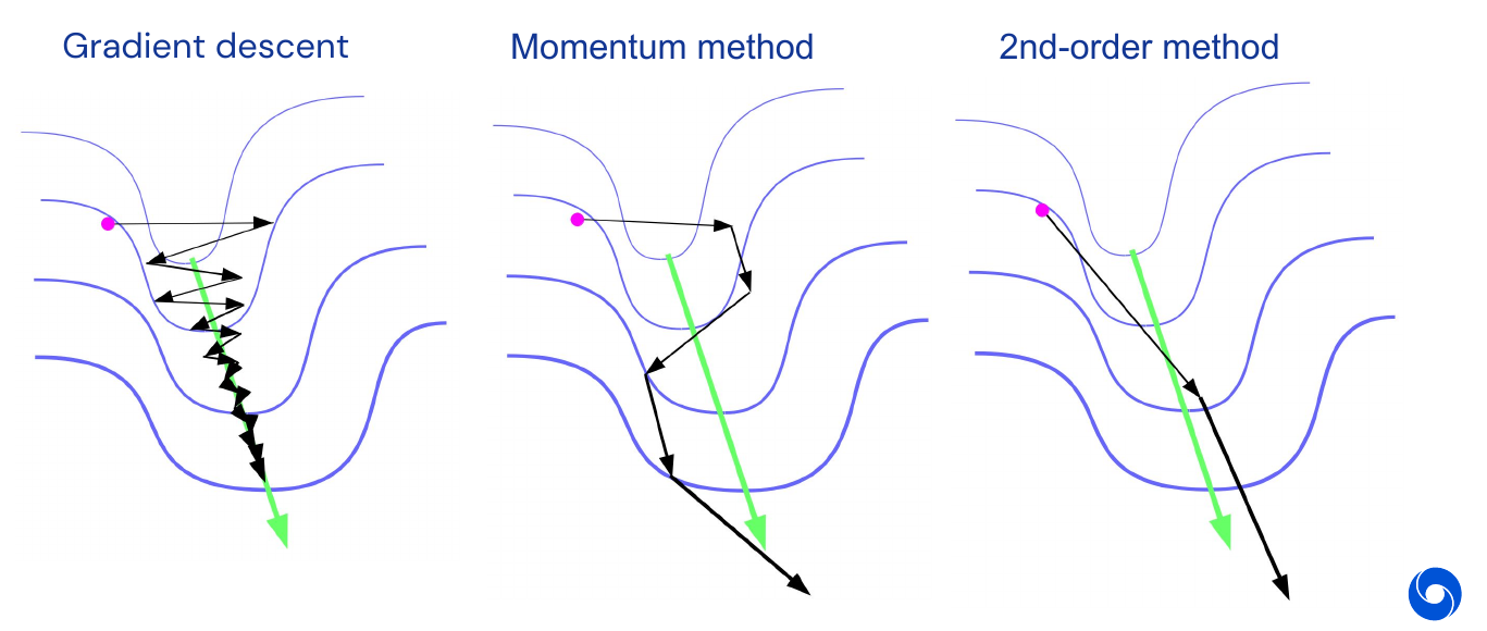
\[\theta_{k+1} = \theta_k - H(\theta)^{-1} \nabla h(\theta_k)\]

Using the second-order Taylor series is the easiest but not necessarily the best way. One can also add momentum into this, but this can’t help if you have a perfect second order method, however it is still used in practice. In the previous valley example the second-order method would clearly perform best:

How does it compare to gradient descent? For gradient descent the maximum allowable global learning rate to avoid divergence is \(\alpha = \frac{1}{L}\) where L is the Lipschitz constant (or maximum curvature). Gradient descent is implicitly minimizing a bad approximation of the second-order Taylor series:

\[\begin{align} h(\theta +d) &\approx h(\theta) + \nabla h(\theta)^T d + \frac{1}{2} d^T H(\theta)d \\ &\approx h(\theta) + \nabla h(\theta)^T d + \frac{1}{2} d^T (LI)d \end{align}\]

Where I is the \(n\)-dimensional identity matrix. This basically assumes that the curvature is maximal in every direction, which is a very pessimistic assumption of \(H(\theta)\).

However there are some issues with the local quadratic approximation:

• The Quadratic approximation of an objective is only correct in a very local region (often neglected)
• Curvature can be approximated to optimistically in a global sense (gradient descent doesn’t have the issue because it takes the global maximum curvature)
• Newtons method uses the Hessian \(H(\theta)\) which may become an underestimate in the region once we take an update step

The solution is to restrict update \(d\) into region \(R\) where approximation is good enough, however the implementation of this is tricky.

Trust-Regions and Dampening

Take a region \(R\) as an \(r\) ball: \(R = \lbrace d: \| d \|_2 \leq r \rbrace\). Then computing

\[\text{arg min}_{d \in R} \bigg(h(\theta) + \nabla h(\theta)^T d + \frac{1}{2} d^T H(\theta)d\bigg)\]

is often equivalent to

\[-(H(\theta) + \lambda I)^{-1} \nabla h(\theta) = \text{arg min}_d \bigg(h(\theta) + \nabla h(\theta)^T d + \frac{1}{2} d^T H(\theta + \lambda I)d\bigg)\]

for some \(\lambda\). Where \(\lambda\) depends on \(r\) in a complicated way, but we can work with \(\lambda\) directly (no need to worry about that in practice).

Remark: This point here is not entirely clear to me. The minimum in some region \(R\) is often the same as to the global approximation \(H(\theta)\) plus some lambda?

The Hessian \(H(\theta)\) is not always the best quadratic approximation for optimization. No one uses the Hessian in neural networks, it is local optimal, for a second-order Taylor series, but that might not be what we want. We would like a more global view, a more conservative approximation.

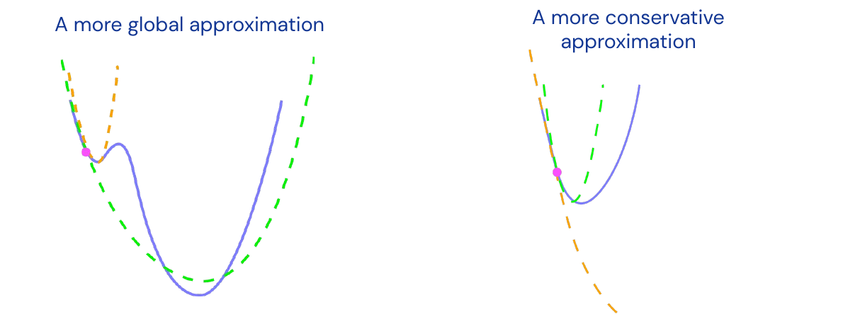
Most important families of related examples are:

• Generalized Gauss-Newton matrix (GGN)
  Remark: I was unable to find a brief and meaningful definition of GGN, for the interested reader there is an in-depth paper from the lecturer about all the topics covered in this part, including a discussion of GGN.

• Fisher information matrix (often equivalent to first)

  Remark: Definition of the Fisher information matrix for those (like me) who are not terribly familiar with it: Let \(\lbrace P_{\theta} \rbrace \: {\theta \in \Theta}, \Theta \subset \mathcal{R}^n\) denote a parametric family of distributions on a space \(\mathcal{X}\). Assume each \(P_{\theta}\) has a density given by \(p_{\theta}\). Then the Fisher information associated with the model is the matrix given by

  \[I_{\theta} = \mathbb{E} \bigg[\nabla \log\big(p_{\theta}(X)\big) \nabla \log \big(p_{\theta}(X)\big)^T\bigg]\]

  Intuitively the Fisher information captures the variability of the gradient \(\log(p_{\theta})\)

• “Empirical Fisher” (cheap but mathematically dubious)

They have nice properties:

• Always positive semi-definite (no negative curvature, would mean you can go infinitely far).
• Give parametrization invariant updates in small learning rate limit (not like Newton).
• Empirically, it works better in practice for neural network optimization (not that clear why).

Problems when applying second-order method for neural networks,

• \(\theta\) can have 10s of millions of dimensions.
• Can not compute, store or invert an \(n \times n\) matrix.
• Hence we must make approximations of the curvature matrix for computation, storage, and inversion.

This is typically done by approximating the full matrix with simpler form.

Diagonal Approximation

The simplest approximation is the diagonal approximation which zeros out all the non-diagonal elements. Inversion is then easy and \(\mathcal{O}(n)\). The computational cost depends on form of original matrix, might be easy or hard. However it is unlikely to be accurate, but can compensate for basic scaling differences between parameters. Used in RMS-prop and Adam methods to approximate Empirical Fisher matrix. It is a very primitive approximation, only works if axis aligned scaling issues appear, normally curvature is not axis-aligned.

Block-Diagonal Approximations

Blocks could correspond to all the weights going in and out of a given unit, or all the weights of one layer. here the Storage cost for a block of size \(b\) is \(\mathcal{O}(bn)\), and the inversion cost is \(\mathcal{O}(b^2n)\). This is only realistic for small block sizes, as one layer can still be in the millions of parameters. This has not been a popular approach for the past couple of years. One well-known example developed for neural networks is TONGA.

Remark: More details on TONGA can be found here.

Kronecker-Product Approximations

It is block-diagonal approximation of GGN/Fisher where blocks correspond to network layers. But each block is approximated by Kronecker product for two smaller matrices.

\[A \otimes C = \begin{pmatrix} [A]_{1,1} C & \dots & [A]_{1, k} C \\ \vdots & \ddots & \vdots \\ [A]_{k,1}C & \dots & [A]_{k,k} C \end{pmatrix}\]

Has storage cost of more than \(\mathcal{O}(n)\), but not that much more (slides are wrong). Apply inverse of \(\mathcal{O}(b^{0.5} n)\), could still be very large, for example for one million parameters this will be a thousand. Currently used in most powerful but heavyweight optimizer, K-FAC.

Remark: Refresh of how the Kronecker-product works: If \(A\) is an \(m \times n\) matrix and \(B\) is a \(p \times q\) matrix, then the Kronecker product \(A \otimes B\) is the \(pm \times qn\) matrix:

\[A \otimes B = \begin{pmatrix} a_{11} B & \dots & a_{1n} B \\ \vdots & \ddots & \vdots \\ a_{m1}B & \dots & a_{mn} B \end{pmatrix}\]

05 - Stochastic Methods - 52:54

So far everything was deterministic, because intuition is easier to build in that case. Why use stochastic methods? Typical objectives in machine learning are an average overall training cases:

\[h(\theta) = \frac{1}{m} \sum^m_{i=1} h_i(\theta)\]

Number of samples can be very big for \(m \gg 1\). This also means computing the gradient is expensive:

\[\nabla h(\theta) = \frac{1}{m} \sum^m_{i=1} \nabla h_i(\theta)\]

The solution is mini-batching: There is often a strong overlap between different \(h_i(\theta)\). This is especially true early in the learning process and most \(\nabla h_i(\theta)\) will look similar. Randomly subsample a mini-batch of training cases \(S \subset \lbrace 1, \dotsc, m \rbrace\) of size \(b << m\) and estimate the gradient as the mean of the subsample:

\[\hat{\nabla} h(\theta) = \frac{1}{b} \sum_{i \in S} \nabla h_i(\theta)\]

So stochastic gradient descent is the same as gradient descent but with mini-batch. We replace the gradient with the stochastic gradient estimate and the procedure becomes stochastic gradient descent (SGD):

\[\theta_{k+1} = \theta_k - \alpha_k \hat{\nabla} h(\theta_k)\]

To ensure convergence, we need to do one of the following:

• Decay the learning rate:

  \[\alpha_k = \frac{1}{k}\]

• Use Polyak averaging, taking an average of all the parameter values visited in the past:

  \[\overline{\theta}_k = \frac{1}{k+1} \sum^k_{i=0} \theta_i\]

  Or use exponentially decaying average (works better in practice but the theory is not as nice)

  \[\overline{\theta}_k = (1-\beta) \theta_k + \beta \overline{\theta}_{k-1}\]

• Slowly increase the mini-batch size during optimization

The theoretical convergence properties of stochastic methods are not as good, they converge slower than non-stochastic versions. The asymptotic rate for SGD with Polyak averaging is

\[E[h(\theta_k)] - h(\theta^*) \in \frac{1}{2k} \text{tr}\big(H(\theta^*)^{-1} \Sigma\big) + \mathcal{O}\bigg(\frac{1}{k^2}\bigg)\]

where \(\Sigma\) is the gradient estimate of the covariance matrix. The iterations until convergence follow:

\[k \in \mathcal{O}\bigg(\text{tr}(H(\theta^*)^{-1}\Sigma)\frac{1}{\epsilon}\bigg)\]

whereas before we had \(k \in \mathcal{O}(\sqrt{\kappa} \log(\frac{1}{\epsilon}))\). Note that there is no logarithm around the term \(\frac{1}{\epsilon}\) in the stochastic case. This makes the dependency much worse for small epsilon, or very close approximations. It’s the best you can prove in theory due to the intrinsic uncertainty. In practice they do not that badly. Polyak averaging is optimal in the asymptotic sense.

Stochastic Second Order and Momentum Methods

We can use mini-batch gradient estimates for second-order and momentum methods too. The curvature matrices are estimated stochastically using decayed averaging over multiple steps. But no stochastic optimization method that has seen same amount of data can have better asymptotic convergence speed than SGD with Polyak. However pre-asymptotic performance matters more in practice. Hence stochastic second-order and momentum methods can still be useful if

• The loss surface curvature is bad enough
• The mini-batch size is large enough

Generally networks without skip connections, which are way harder to optimize, profit most from second order methods such as K-FAC. This is illustrated in the image below where three optimizers are used to train an image ImageNet classifier. The network is a 100 layers deep CNN without skip connections or batch norm and is carefully initialized.

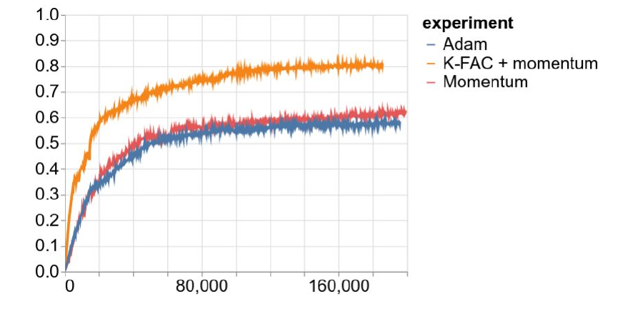
Once you include skip connections and BatchNorm the performance difference disappears. This means that the implicit curvature number of ResNet is pretty good. second-order methods are twice as slow, but with some implementation tricks you can get them to be only 10% slower than first-order methods.

Conclusion and Summary

• Optimization methods: Are the main engine behind neural networks and enable learning models by adapting parameters to minimize some objective
• First-order methods (gradient descent): Take steps in the direction of “steepest descent” but run into issues when curvature varies strongly in different directions
• Momentum methods: Use principle of momentum to accelerate along directions of lower curvature and obtain “optimal” convergence rates for first-order methods
• Second-order methods: Improve convergence in problems with bad curvature. But they require use of trust-regions and the curvature matrix approximations need to be practical in high dimensions (e.g. for neural networks)
• Stochastic methods: Have slower asymptotic converge but pre-asymptotic convergence can be sped up using second-order methods and/or momentum

Overall we can make make networks easier to optimize with architectural choices or make optimization better. Even though currently network optimization works well with first-order methods, for new classes of models we might need better optimization methods.

Questions - 1:11:30

• On Initialization: It is very hard and a deep subject, there are new results upcoming this year. For now every initialization starts with the basic Gaussian factor. Becomes important when not using batch norm or skip connections
• On BatchNorm and ResNet: they make the network look linear in beginning, so its easy to optimize in beginning and only adds complexity over time
• On Regularization: Not important these days, should not rely on optimizer to do regularization
• On condition number: No one measures condition number in practice, and it would not capture the essence (some dimensions might be completely flat)
• On new emergent research: if you start with good initialization, neural networks loss surface will look quadratically convex in your neighborhood and you can get to zero error (global minimum) with the above mentioned techniques
• On the reason for lowering learning rate or Polyak averaging: it is inversely related to batch size (larger batch size reduces gradient variance estimate, so there is less need for those techniques.). When you double the batch size, you can double the learning rate (as a naive rule)

Highlights

• See gradient descent as linear or quadratic approximation by using Taylor series in small neighborhood
• Optimality for various methods, especially SGD with Polyak in stochastic case
• ResNet and especially skip connections make the optimization problem much easier currently
• This line of research might become highly important again once we use different network building blocks

Episode 6 - Sequences and Recurrent Neural Networks

01 - Motivation - 1:31

So far we always used vectors and images as inputs, now we will look at sequences. They are a collection of elements where

• Elements can be repeated
• Order matters
• Length is variable (potentially infinite)

Sequences are everywhere: words, letters, speech, videos, images, programs, decision making.

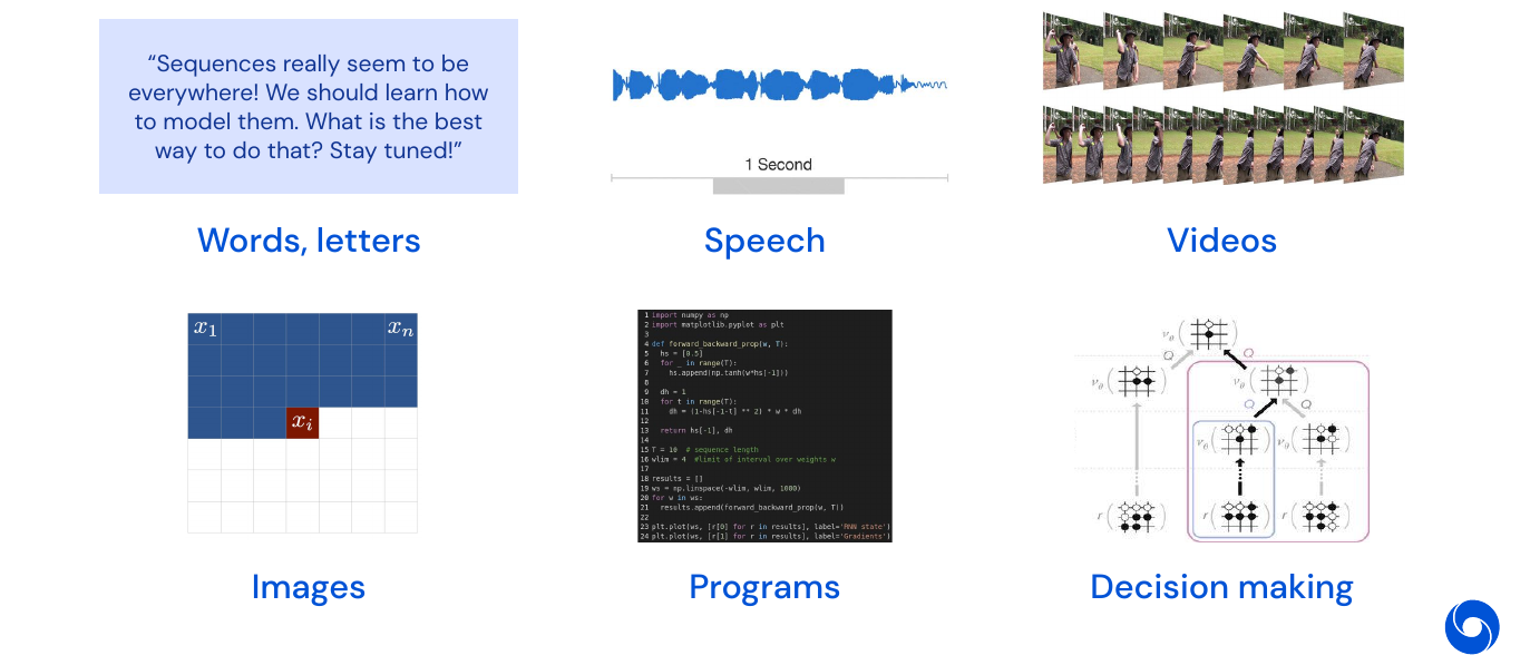
The models we have seen so far don’t do well with sequential data.

02 - Fundamentals - 5:24

When training machine learning models, the four basic questions to answer are: data, model, loss and optimization for the supervised case. For sequences we have:

• Data: a sequence of inputs

  \[\lbrace x \rbrace_i\]

  In the supervised case we have \(\lbrace x, y \rbrace_i\).

• Model: the probability of a sequence

  \[p(x) \approx f_{\theta}(x)\]

  In the supervised case we have \(y \approx f_{\theta}(x)\).

• Loss: the sum of the log probability of the sequence under the model

  \[L(\theta) = \sum^N_{i=1} \log(p(f_{\theta}(x_i)))\]

  In the supervised case we have \(L(\theta) = \sum^N_{i=1} l(f_{\theta}(x_i), y_i)\).

• Optimization: finding the parameter which minimizes the loss function

  \[\theta^* = \text{arg min}_{\theta} L(\theta)\]

  Which is the same as in the supervised case

Modeling word probabilities is really difficult. The simplest model would be the product of individual words, if we assume independence:

\[p(\mathbf{x}) = \prod^T_{t=1} p(x_t)\]

But the independence assumption does not match the sequential nature of language. A more realistic model would be to assume conditional dependence of words:

\[p(x_T) = p(x_T \mid x_1, \dotsc, x_{T-1})\]

We could then use the chain rule to compute the joint probability of \(p(\mathbf{x})\) from the conditionals

This is a more realistic model but imagine you model the simple dependence \(p(x_2 \mid x_1)\) as below:

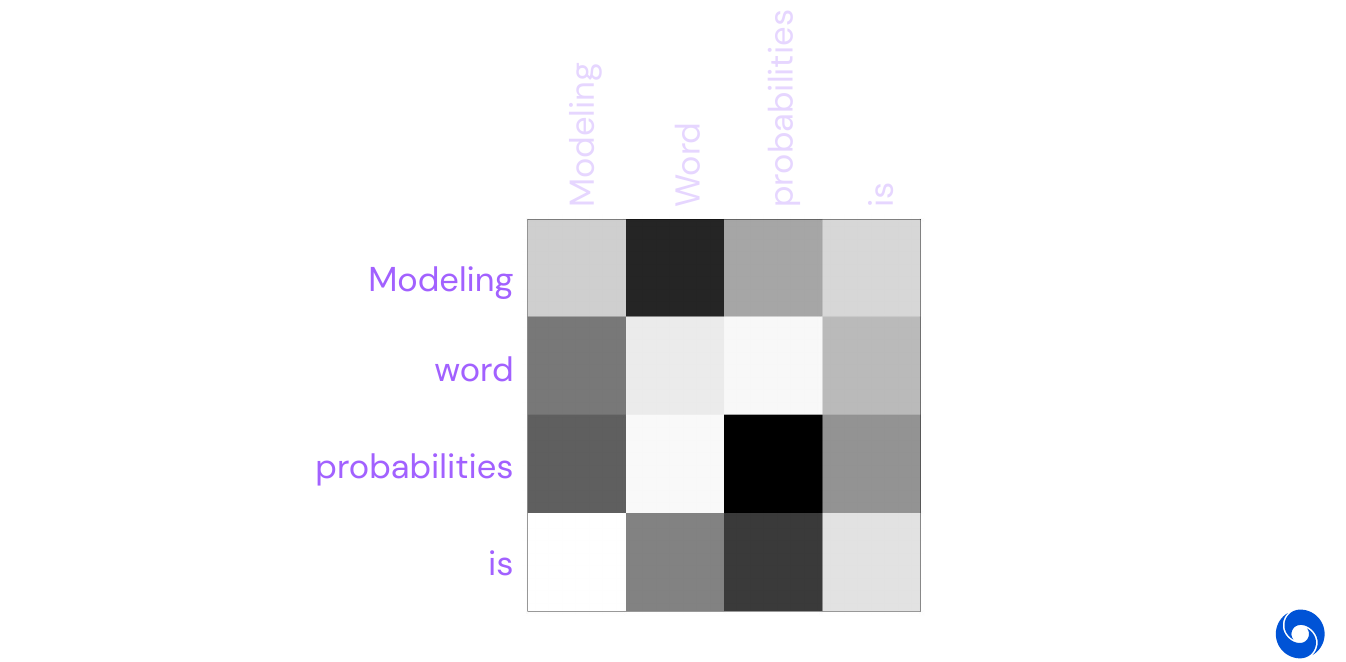
This is only for four words, typically language has thousands of words.

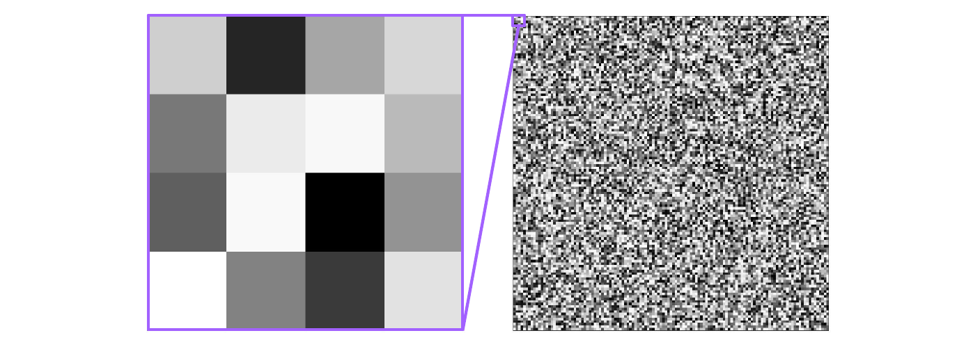
And this is only for a context of size \(N=1\), if you add more context then it will grow with \(\text{vocabulary}^N\). Instead we could fix the window size, called N-grams:

\[p(\mathbf{x}) = \prod^T_{t=1} p(x_t \mid x_{t-N-1}, \dotsc, x_{t-1})\]

It has the downside that it does not take into account words that are more than \(N\) words away, and the data table can still be huge. In summary: modeling probabilities of sequences scales badly.

Can we learn this probability estimation from data in a efficient way? Yes, by vectorizing the context, i.e. we summarize the previous words with the help of a function \(f_{\theta}\) in a state vector \(h\) such that

\[p(x_t \mid x_1, \dotsc, x_{t-1}) \approx p(x_t \mid h)\]

What are desirable properties of \(f_{\theta}\)?

• Order matters
• Variable length
• Differentiable (learnable)
• Pairwise encoding
• Preserves long-term dependencies

How do N-gram and addition score on these properties?

At the same time we want a function \(g_{\theta}\) which is able to model conditional probabilities from the hidden state \(h\)

What are desirable properties of \(g_{\theta}\)?

• Individual changes can have large effects (non-linear/deep)
• Returns a probability distribution

How do we build deep networks that meet these requirements?

Recurrent Neural Networks (RNN)

RNNs can do both at once with two steps:

1. Calculate state variable \(h_t\) from current input \(x_t\) and previous context \(h_{t-1}\):

   \[h_t = \tanh(W_h h_{t-1} + W_x x_t)\]

2. Predict the target \(y\) (next word) from the state \(h\)

   \[p(y_{t+1}) = \text{softmax}(W_y h_t)\]

Where \(W_h, W_x, W_y\) are three weight matrices which are shared over all steps.

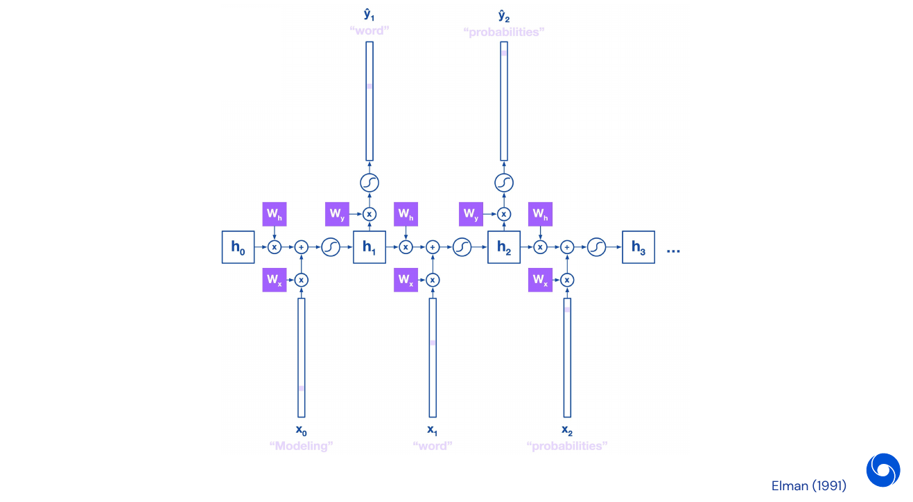
We can unroll RNNs to do back-propagation. As loss we use cross-entropy for each word output, as word prediction is a classification problem where the number of classes is the size of the vocabulary:

• Loss for one word: \(L_{\theta}(y, \hat{y})_t = -y_t \log(\hat{y}_t)\)
• Loss for the sentence: \(L_{\theta}(y, \hat{y}) = - \sum^T_{t=1} y_t \log(\hat{y}_t)\)

For parameters \(\theta = \lbrace W_h, W_x, W_y \rbrace\). We have to calculate the derivative of the loss function with respect to each of them. Starting with \(W_y\) we get:

\[\frac{\partial L_{\theta, t}}{\partial W_y} = \frac{\partial L_{\theta, t}}{\partial \hat{y}_t} \frac{\partial \hat{y}_t}{\partial W_y}\]

For the derivative with respect to \(W_h\) the case is a bit more complicated as we have to unroll over time:

\[\frac{\partial L_{\theta, t}}{\partial W_h} = \frac{\partial L_{\theta, t}}{\partial \hat{y}_t} \frac{\partial \hat{y}_t}{\partial h_t} \frac{\partial h_t}{\partial W_h}\]

where

\[\begin{align} \frac{\partial h_t}{\partial W_h} &= \frac{\partial h_t}{\partial W_h} + \frac{\partial h_t}{\partial h_{t-1}} \frac{\partial h_{t-1}}{\partial W_h} \\ &= \frac{\partial h_t}{\partial W_h} + \frac{\partial h_t}{\partial h_{t-1}} \bigg[ \frac{\partial h_{t-1}}{\partial W_h} + \frac{\partial h_{t-1}}{\partial h_{t-2}} \frac{\partial h_{t-2}}{\partial W_h}\bigg] \\ &= \dotsc \\ &= \sum^t_{k=1} \frac{\partial h_t}{\partial h_k} \frac{\partial h_k}{\partial W_h} \end{align}\]

Putting this back together with the initial formula we get

\[\frac{\partial L_{\theta, t}}{\partial W_h} = \frac{\partial L_{\theta, t}}{\partial \hat{y}_t} \frac{\partial \hat{y}_t}{\partial h_t} \frac{\partial h_t}{\partial W_h} = \sum^t_{k=1} \frac{\partial L_{\theta, t}}{\partial \hat{y}_t} \frac{\partial \hat{y}_t}{\partial h_t} \frac{\partial h_t}{\partial h_k} \frac{\partial h_k}{\partial W_h}\]

However the longer we have to unroll a RNN, the more problems we get with vanishing gradients. Consider the following example:

This leads to the following problems:

\[\begin{align} h_t &= W_h h_{t-1} & h_t \longrightarrow \infty \text{ if } \mid W_h \mid > 1 \\ h_t &= (W_h)^t h_0 & h_t \longrightarrow 0 \text{ if } \mid W_h \mid < 1 \end{align}\]

Remark: In the first case we can do gradient clipping to stabilize the gradient.

While the values are bounded by \(\tanh\) the gradients are still affected by it. It does not give a gradient if the value is not close to \(-1\) or \(1\).

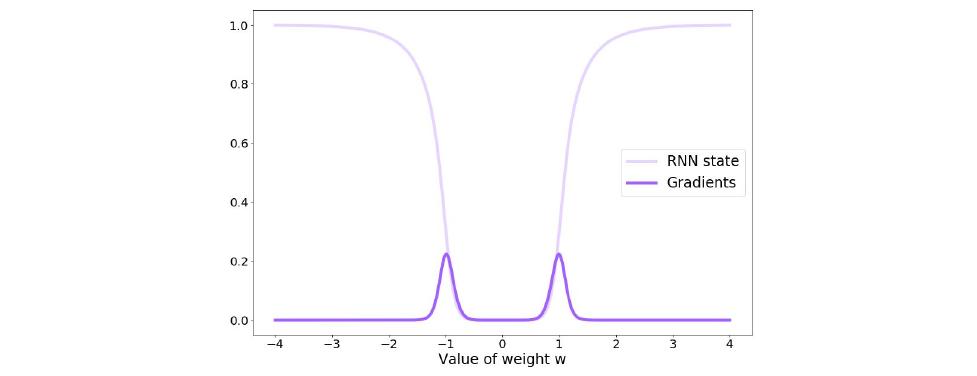
Summarizing the properties of RNNs, they can model variable length sequences and can be trained via back-propagation. However they suffer from the vanishing gradients problem which stops them from capturing long-term dependencies.

So how can we still capture long-term dependencies?

Long Short-Term Memory (LSTM) Networks

The architecture in the image below describes a LSTM cell. Note that here there are two states which are propagating between individual cells, we have the hidden state \(h_t\) and additionally a cell state \(c_t\).

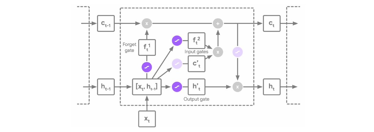
An LSTM has three main pathways:

1. Forget gate:

   \[f_t^1 = \sigma(W_{f^1} [h_{t-1}, x_t] + b_{f^1})\]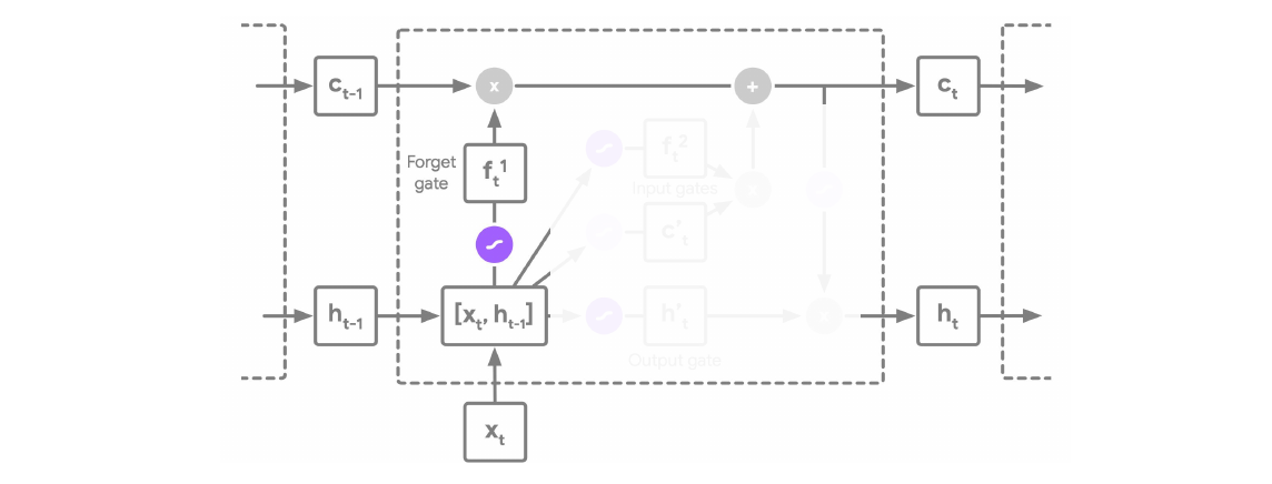

   

2. Input gates:

   \[f^2_t = \sigma(W_{f^2}[h_{t-1}, x_t] + b_{f^2} ) \odot \tanh(W_{f^2} [h_{t-1}, x_t] + b_{f^2})\]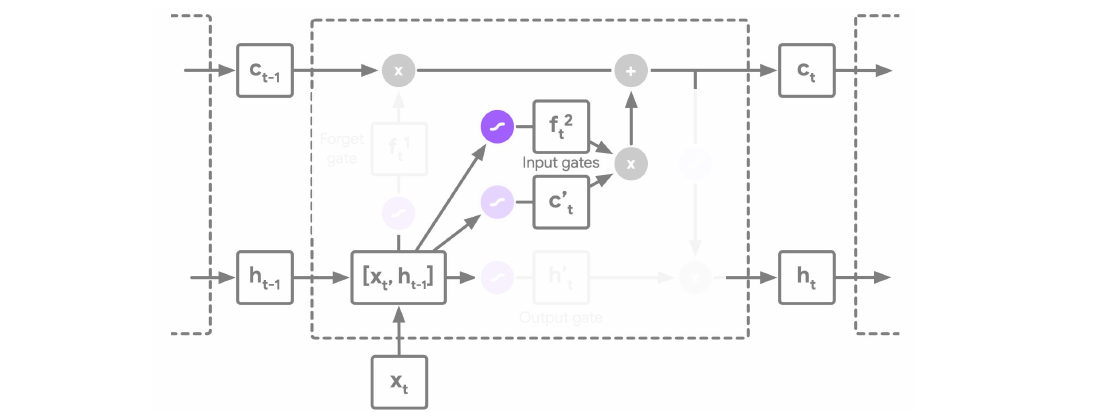

   

3. Output gate:

   \[h^*_t = \sigma(W_{h^*_t} [h_{t-1}, x_t] + b_{h^*_t}) \odot \tanh(c_t)\]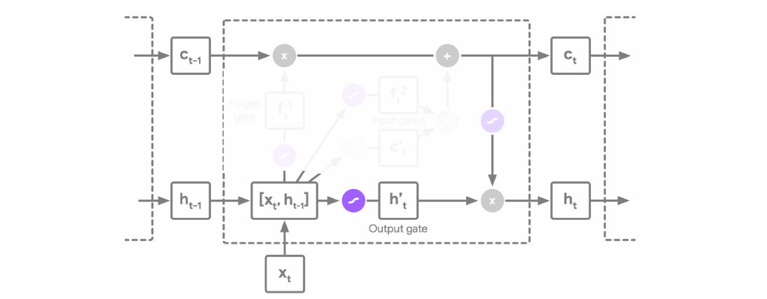

   

Remark: The explanation here why LSTM solve the vanishing gradient problem did not seem very clear from the speaker. From my understanding the vanishing gradient problem disappears because the gradient has an alternative path, it can flow through the \(c_t\). There are no \(\tanh\) or \(\sigma\) functions between \(c_{t-1}\) and \(c_t\) which could shrink the gradient. Hence they perform a similar function to skip connections in a ResNet. For a more detailed explanation on RNNs and LSTMs I recommend the excellent Standford lecture on RNNs.

LSTM overcome the vanishing gradient problem by the use of gating mechanisms and solve the long-range dependency problem.

03 - Generation - 43:46

So far we focused on optimizing the log probability estimates produced by the model:

\[L_{\theta}(y, \hat{y})_t = - y_t \log(\hat{y}_t)\]

We could use the trained model to evaluate the probability of a new sentence. Or even better, we can use it to generate a new sequence: start with a word and use the sampled \(\hat{y}\) as input for the next iteration of the network.

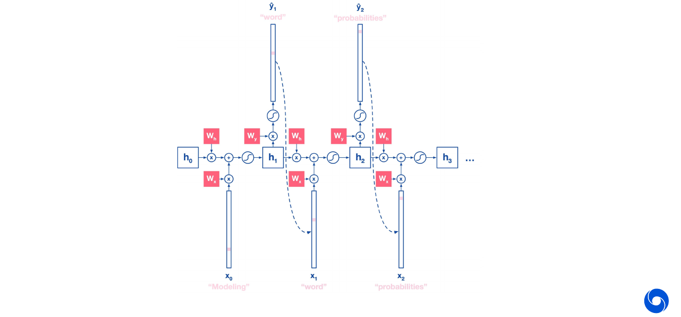
Use the argmax of the output to decide which word was sampled.

Images as Sequences PixelRNN

We can also see an image as a sequence of pixels, which depends on all the values which have been sampled before. We start from the top left and go over all the lines.

We can do this in the same way as generating a sequence, sample with the softmax over the entire image, start on top left. It can be interesting to look at the distribution for each pixel. It produces decently looking images, but not great compared to state of the art methods.

Natural Languages as Sequences

Sequence-to-sequence models can also be used for translation, start with English words and use them as initial state, then start outputting Japanese words.

There is more than one way to create sequences, from one-to-one to many-to-many.

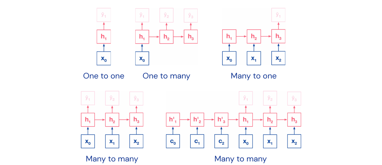
Google Neural Machine Translation: has an encoder and decoder structure. This architecture almost closed the gap between human and machine translation.

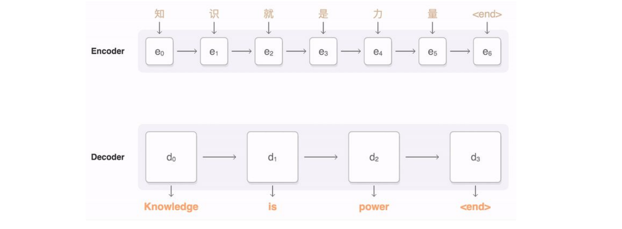
Image captioning: start with features from an image passed trough a CNN, then feed the features as hidden state into a RNN.

Audio Waves as Sequences

We can see audio waves as sequences and apply convolutions. This is mostly done using dilated convolutions, to predict one signal at a time. This structure allows for taking into account various time scales.

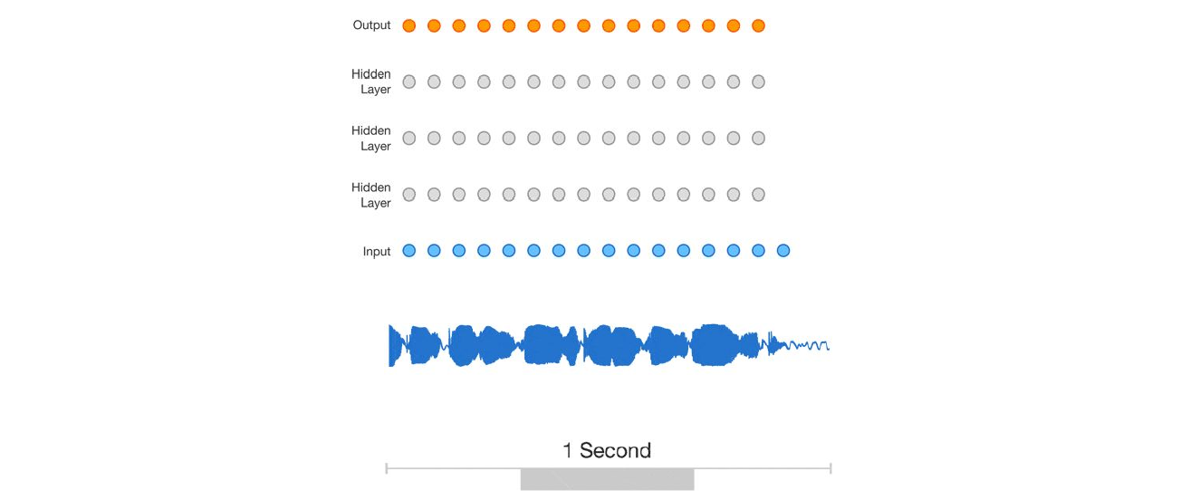
We can even put these models in the same table as before and compare it to RNN and LSTMS:

Policies as Sequences

We can see reinforcement learning policies as sequences, which can be applied in many places. One example would be where to draw on a canvas. Another one is OpenAI five and AlphaStar playing games using LSTM.

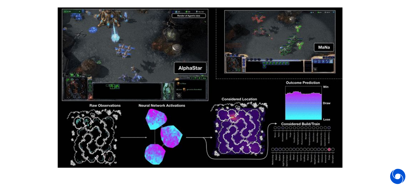
The image below shows the AlphaStar architecture in more detail. While a ResNet is used to extract spatial information, the core is an LSTM which fuses inputs from different modalities and decides which actions to take. It keeps track of the state of the game.

Attention for Sequences: Transformers

What is the difference between a transformer and a convolution architecture? The transformer is connected to every input which is weighted by attention (we will see more details in a later lecture).

An example of a transformer architecture is GPT-2 which adapts to style and content. It has 1.5 billion parameters and was trained on a dataset of 40GB of text data from eight million websites. The transformer is finally an architecture which fulfills all the criteria:

Questions - 1:11:51

• Do models focus only on local consistency? Could be mixed with a memory module to incorporate truly long term connections, need more hierarchy in the model.
• Deep learning is hard to reconcile with symbolic learning, reasoning level is hard to measure. Can’t see if it learns concepts.
• No constraints on hidden states, hard to interpret how they are working. Very model specific. Also hard to get an intuitive understanding.

Highlights

• Nice gradient calculation to show vanishing gradients in RNN
• Overview of properties and different models (RNN, LSTM, Conv, Transformers)

Conclusion of first half of the course

The breadth of the lectures is amazing, there are a lot of topics covered. Sometimes it would be good if there was a bit more depth, as some of the topics feel a bit rushed. However the trade-off between depth and breadth is understandably a difficult one to make. Unfortunately the audience questions are almost impossible to understand, it would help if the lecturer would repeat them quickly for the audience.

References

A list of resources used to write this post, also useful for further reading:

• DeepMind x UCL Deep Learning Lecture Series 2020 for the lectures, each video also has a link to the slides in the description
• Convolutional Neural Networks for Visual Recognition for the Stanford lecture on very similar topics but with more depth in various places
• DeepMind YouTube channel for more lectures and talks. Among others there are classes on reinforcement learning and an older version of the deep learning lectures from 2018

Comments

I would be happy to hear about any mistakes or inconsistencies in my post. Other suggestions are of course also welcome. You can either write a comment below or find my email address on the about page.