Recently I came across a paper extensively using the EM algorithm and I felt I was lacking a deeper understanding of its inner workings. As a result I decided to review it here, mostly following the excellent machine learning class from Stanford CS229. In this post I follow the structure outlined in the class notes but change the notation slightly for clarity. We will first have a look at \(k\)-means clustering, then see the EM algorithm in the special case of mixtures of Gaussians and finally discover a general version of EM.

Basic Concepts and Notation

Readers familiar with the basic concepts and notation in probability theory may skip this section.

• Scalar: A scalar \(a \in \mathbb{R}\) is a single number. Usually denoted in lower case.

• Vector: A vector \(v \in \mathbb{R}^n\) is a collection of \(n\) scalars, where \(n>0\) is an integer.

  \[v=\begin{pmatrix} v_{1} \\ v_{2} \\ \vdots \\ v_{n} \\ \end{pmatrix}\]

  For this post we will not denote vectors in bold, as we are almost exclusively dealing with vectors. I hope the difference between vectors and scalars will still be clear from the context.

• Random Variable: A variable whose values depend on the outcomes of a random phenomenon, we usually denote it by \(X\) (upper case) and an outcome by \(x\) (lower case). An example would be a random variable X which represents a coin throw, it can take value zero for head or one for tail.

• Probability Distribution: A function \(p\) associated with a random variable \(X\), it will tell us how likely an outcome \(x \in X\) is. In the case of a fair coin, we will have

  \[P(X=0) = p_X(0) = p_X(1) = P(X=1) = \frac{1}{2}\]

  We usually omit the subscript \(p_X\) and only write \(p\) for simplicity. Often we will also that a probability distribution is parametrized by a vector \(\theta \in \mathbb{R}^n\), in that case we will write \(p_{\theta}\) to make the dependence clear.

• Expectation: For a random variable \(X\) the expectation is defined as

  \[\mathbb{E}[X] := \sum_{x \in X} p(x) x\]

  A weighted average of all the outcomes of a random variable (weighted by the probability). The expectation of the coin throw example is \(\mathbb{E}[X] = 0 \cdot p(0) + 1 \cdot p(1) = 0 \cdot \frac{1}{2} + 1 \cdot \frac{1}{2} = \frac{1}{2}\).

• Mean: Let \(n \geq 1\) and \(x_1, \dotsc , x_n \in \mathbb{R}\), the mean of \(x_1, \dotsc , x_n\) is

  \[\mu = \frac{1}{n}\sum_{i=1}^n x_i\]

• Variance: Let \(n \geq 1\), \(x_1, \dotsc , x_n \in \mathbb{R}\) and \(\mu\) the mean that sequence. Then the variance of \(x_1, \dotsc , x_n\) is defined to be

  \[\sigma^2 = \frac{1}{n}\sum_{i=1}^n (x_i -\mu)^2\]

• Normal Distribution: The normal or Gaussian distribution \(N(\mu, \sigma^2)\) for \(\mu, \sigma \in \mathbb{R}\) has the density

  \[f(x) = \frac{1}{\sigma \sqrt{2\pi}} e^{-\frac{1}{2}\big(\frac{x-\mu}{\sigma}\big)^2}\]

  We call it the standard normal distribution if \(\mu =0\) and \(\sigma^2=1\). Some of the important properties are best seen visually:

  

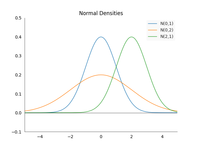
  The density is always centered at the mean \(\mu\) and symmetric around it. The larger \(\sigma^2\), the more spread out the density will be. \(67\%\) of the area under the density in between \(-\sigma^2\) and \(\sigma^2\).

• Maximum Likelihood Estimation: For a probability distribution \(p_\theta\) with parameter \(\theta\) and data \(\lbrace x_1, \dotsc, x_n \rbrace\) we can estimate \(\theta\) by maximizing the probability over the data:

  \[\theta = \text{arg} \max_{\theta} p_{\theta}(x) = \prod_{i=1}^n p_{\theta}(x_i)\]

  This is called maximum likelihood estimation. Often it is more convenient to maximize the log likelihood instead, and because the log is a strictly increasing transformation the result will not change. The log transformation has the additional benefit that the product becomes a sum:

  \[\theta = \text{arg} \max_{\theta} \log(p_{\theta}(x)) = \sum_{i=1}^n \log(p_{\theta}(x_i))\]

  Which is beneficial when doing numerical optimization.

• Supervised Learning: The scenario of supervised learning is when data of the form \((x_i, y_i)\) is available, we have an input \(x_i\) and expect a model to produce output \(y_i\) for \(i \in \lbrace 1, \dotsc, n \rbrace\). Where the input and output can be in arbitrary spaces. A common example in computer vision is input images \(x_i \in \mathbb{R}^{h \times w}\) and output labels which are one hot encoded in \(k\) categories, \(y_i \in \lbrace 0, 1 \rbrace^k\).

• Unsupervised Learning: In the scenario of unsupervised learning we only have data \((x_i)\) but no associated labels for \(i \in \lbrace 1, \dotsc, n \rbrace\).

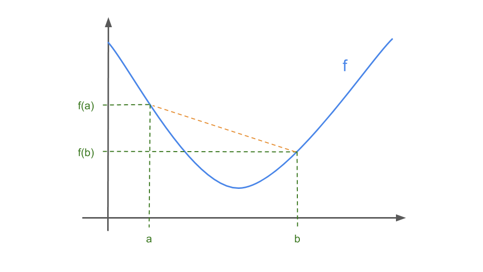
• Convex Function: a function \(f : \mathbb{R} \longrightarrow \mathbb{R}\) is called convex if

  \[\forall x, y \in \mathbb{R}, \forall \alpha \in [0,1]: f(\alpha x + (1-\alpha)y) \leq \alpha f(x) + (1-\alpha) f(y)\]

  Alternatively \(f\) is convex if and only if \(f''(x) \geq 0 \: \forall \: x \in \mathbb{R}\). In visual terms, if you connect any two points on the function with a straight line, you will be guaranteed to be above the function (see the orange line).

  

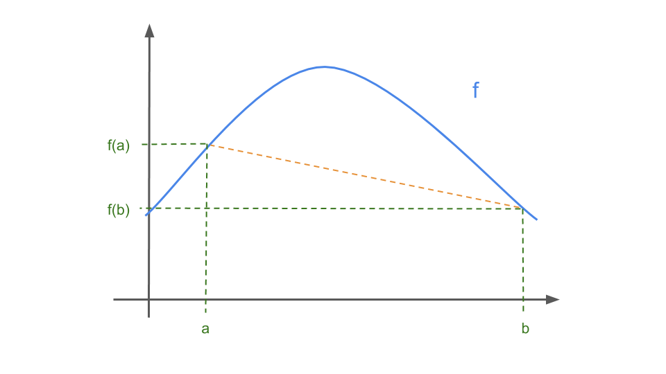
• Concave Function: a function \(f : \mathbb{R} \longrightarrow \mathbb{R}\) is called convex if

  \[\forall x, y \in \mathbb{R}, \forall \alpha \in [0,1]: f(\alpha x + (1-\alpha)y) \geq \alpha f(x) + (1-\alpha) f(y)\]

  or alternatively, \(f\) is concave if and only if \(-f\) is convex. In visual terms, if you connect any two points on the function with a straight line, you will be guaranteed to be below the function (see the orange line).

  

• Jensen’s Inequality: Let \(f : \mathbb{R} \longrightarrow \mathbb{R}\) be a convex function, and let \(X\) be a random variable. Then

  \[\mathbb{E}[f(X)] \geq f(\mathbb{E}[X])\]

  For two points Jensen’s inequality boils down to almost the same image as the one for a convex function:

  

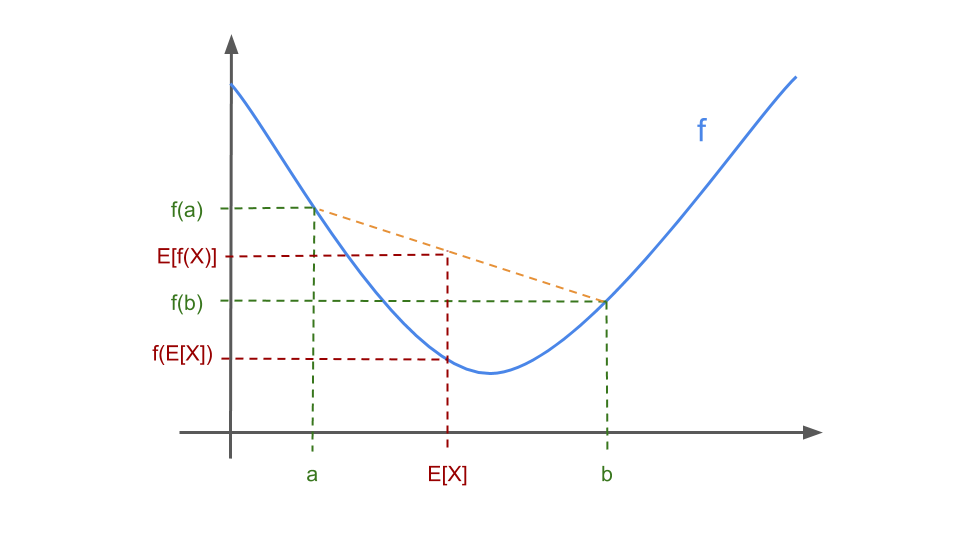
  The theorem tells us that the inequality is true for a arbitrary combination of points on the function \(f\), as long as the weights of the points sum up to one.

\(K\)-Means Clustering

Let us start with the clustering problem, where we are trying to group \(n\) data points \(x_1, \dotsc, x_n \in \mathbb{R}^d\) into \(k\) groups. This is a case of unsupervised learning, so we have no ground truth labels \(y_i\) available. We will assign a one-hot encoded class variable \(c_i \in \lbrace 0, 1 \rbrace^k\) to each input \(x_i\) according to the rules specified in the algorithm below. The \(k\)-means algorithm is a way of doing this so we group \(x_i\)’s that are close together, in this case close means in Euclidean distance. The algorithm works as follows:

1. Initialize cluster centroids \(\mu_1, \dotsc, \mu_k \in \mathbb{R}^d\) randomly

2. Repeat until convergence:

   1. For every \(i \in \lbrace 1, \dotsc, n \rbrace\):

      \[c_i := \text{arg max}_j \| x_i - \mu_j \|^2\]

      Assign every input vector \(x_i\) to the closest centroid \(\mu_j\).

   2. For every \(j \in \lbrace 1, \dotsc, k \rbrace\):

      \[\mu_j := \frac{\sum^n_{i=1} 1_{c_i = j} x_i}{\sum^n_{i=1} 1_{c_i = j}}\]

      Update every centroid \(\mu_j\) as average of all input vectors \(x_i\) assigned to centroid \(j\).

The number of clusters \(k\) has to be chosen by the user of the algorithm. There is no “right” value for it, it is a hyper parameter and depends on the problem one is trying to solve. In practice it is common to select the \(k\) initial centroids randomly from the data. Here is an illustration of the process for \(k=2\).

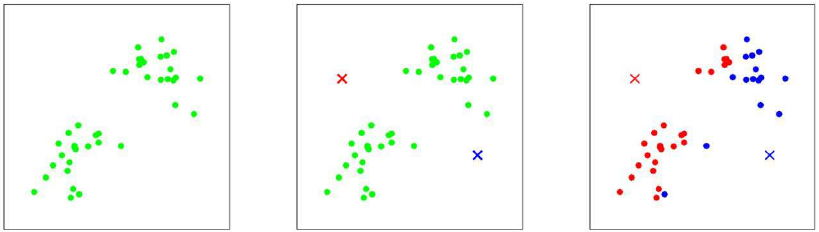
The left image shows the initial state with no centroids and no input points assigned to any cluster. We set \(k=2\) and chose two random points as the centroids in the middle image. On the right side we do the first assign step, every point is colored according to the closest centroid.

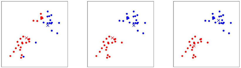
The left image shows the first update step, the centroids move into the center of the input data assigned to them. Then follows another assign step in the middle image, the two groups are now already separated by color. The right image shows what happens after another update. The centroids are now in the center of their groups. We could stop the algorithm now as any successive updates would not change the assignments of points to centroids nor the position of the centroids.

How would we analytically measure what we just described? One way to measure convergence is the distortion function:

\[J(c, \mu) = \sum^n_{i=1} \| x_i - \mu_{c_i} \|^2\]

Where \(c\) and \(\mu\) are the collection of all class vectors and centroids, i.e. \(c = (c_1, \dotsc, c_n)\) and \(\mu = (\mu_1, \dotsc, \mu_k)\) . It measures the sum of squared distances between each example \(x_i\) and its associated centroid \(\mu_{c_i}\). It can be shown that \(k\)-means clustering is coordinate ascent on \(J\). It monotonically decreases when \(k\)-means is applied, which usually implies that \(c\) and \(\mu\) will converge too. In theory it is possible that \(k\)-means oscillates between different clusterings, but that almost never happens in practice.

However the distortion function \(J\) is non-convex, so we are not guaranteed to converge to a global optimum. Hence if we apply \(k\)-means only once, we might get stuck in a local optimum. To increase the chances of finding a global minimum, we can run the algorithm multiple times with different random initializations and then pick the result with the lowest value in the distortion function \(J\). There is also no guarantee how fast \(k\)-means will converge.

EM-Algorithm for Mixtures of Gaussians

So far for the \(k\)-means case we had the implicit assumption that each input sample \(x_i\) can only belong to one centroid \(\mu_j\). What if we relax that assumption and instead assign weights for each input and centroid pair? Let \(w_{ij}\) be the weight that input \(x_i\) gives to centroid \(\mu_j\). If we assume that these weights are normalized, i.e. \(1 = \sum_i w_{ij}\) we can call them a probability. Then the weight \(w_{ij}\) is the probability that input \(x_i\) belongs to centroid \(\mu_j\). We can model this with a random variable \(z_i \sim \text{Multinomial}(\phi)\) and have \(w_{ij} = P(z_i = j \mid x_i)\). Note that the \(z_i\)’s are latent variables, they are not unobservable.

We would also like a more flexible notion of a cluster, so far the cluster was extending equally in all directions. The clusters always had the form of a circle, we can generalize this by also making ellipses possible. A mathematically formal way to describe this is to say samples \(x_i\) from a cluster \(j\) follow a normal distribution with mean \(\mu_j\) and covariance matrix \(\Sigma_j\), i.e. \(x_i \mid z_i = j \sim N(\mu_j, \Sigma_j)\). Note that each cluster has its own covariance matrix.

Putting the two previous points together, we get a joint distribution \(p(x_i, z_i)\) of the problem, a mixture of Gaussians model. We can factorize the joint distribution as conditional and marginal distribution:

\[p(x_i, z_j) = p(x_i | z_j)p(z_j) = p_{\mu, \Sigma}(x_i | z_j)p_{\phi}(z_j)\]

The right hand side are the two distributions we defined above. We note that the problem is parametrized by \(\mu\), \(\Sigma\) and \(\phi\). We would normally estimate these maximizing the log likelihood of the data:

\[\begin{align*} l(\mu, \Sigma, \phi) &= \sum^n_{i=1} \log \big(p_{\mu, \Sigma, \phi}(x_i)\big) \\ &= \sum^n_{i=1} \log\Bigg(\sum^k_{j=1}p_{\mu, \Sigma, \phi}(x_i, z_j)\Bigg) \\ &= \sum^n_{i=1} \log \Bigg(\sum^k_{j=1} p_{\mu, \Sigma}(x_i | z_j)p_{\phi}(z_j) \Bigg) \end{align*}\]

However in this case it is not possible to find the maximum likelihood with the usual method, setting the derivatives to zero and solve it with respect to the parameters. There is no solution in closed form, the main problem is the sum in the \(log\) as \(z_i\) is a random variable. Remember that the \(z_i\) indicate from which Gaussian a data point originates. If we would know the true label \(c_i\), the problem would become traceable as the inner sum disappears:

\[\begin{align*} l(\mu, \Sigma, \phi) &= \sum^n_{i=1} \log\big(p_{\mu, \Sigma, \phi}(x_i)\big) \\ &= \sum^n_{i=1} \log \big( p_{\mu, \Sigma}(x_i | z_i = c_i) \big) + \log \big(p_{\phi}(z_i = c_i)\big) \end{align*}\]

This allows maximization with respect to the parameters and results in the following estimates:

\[\begin{align*} \phi_j &= \frac{1}{n} \sum^n_{i=1} 1_{\lbrace z_i = j \rbrace} \\ \mu_j &= \frac{\sum^n_{i=1} 1_{\lbrace z_i = j \rbrace} x_i}{\sum^n_{i=1} 1_{\lbrace z_i = j \rbrace}} \\ \Sigma_j &= \frac{\sum^n_{i=1} 1_{\lbrace z_i = j \rbrace} (x_i - \mu_j)(x_i - \mu_j)^T}{ \sum^n_{i=1} 1_{\lbrace z_i = j \rbrace}} \end{align*}\]

However here the \(z_i\)s are not known, what is the alternative? We can guess the the values of the \(z_i\)’s. This is the first step or E-step of the Expectation-Maximization algorithm:

\[w_{ij} := p_{\mu, \Sigma, \phi}(z_i = j | x_i) \qquad \forall i,j\]

We calculate the posterior probability of our parameters \(z_i\) given an input \(x_i\) using the current setting of parameters \(\mu, \Sigma, \phi\). We have not explicitly defined the density \(p(z \mid x)\) but, using Bayes rule and the law of total probability, we can calculate it with the two known densities \(p(x \mid z)\) and \(p(z)\):

\[\begin{align*} p_{\mu, \Sigma, \phi}(z_i = j \mid x_i) &= \frac{p_{\mu, \Sigma}(x_i \mid z_i = j) p_{\phi}(z_i = j)}{p_{\mu, \Sigma, \phi}(x_i)} \\ &= \frac{p_{\mu, \Sigma}(x_i \mid z_i = j) p_{\phi}(z_i = j)}{\sum^k_{j=1} p_{\mu, \Sigma, \phi}(x_i, z_j)} \\ &= \frac{p_{\mu, \Sigma}(x_i \mid z_i = j) p_{\phi}(z_i = j)}{\sum^k_{j=1} p_{\mu, \Sigma}(x_i \mid z_i = j) p_{\phi}(z_i = j)} \end{align*}\]

The values \(w_{ij}\) calculated in the E-step represent our soft guesses for the values of \(z_i\).

The EM algorithm for Gaussian Mixtures

The EM algorithm for the Gaussian Mixtures case can now be written as below by replacing the hard values \(1_{\lbrace z_i = j \rbrace}\) for \(z_i\) by the soft guesses \(w_{ij}\).

Repeat until convergence:

1. E-Step:

   \[w_{ij} := p_{\mu, \Sigma, \phi}(z_i = j | x_i) \qquad \forall i,j\]

2. M-Step:

   \[\begin{align*} \phi_j &:= \frac{1}{n} \sum^n_{i=1} w_{ij} & \forall j \\ \mu_j &:= \frac{\sum^n_{i=1} w_{ij} x_i}{\sum^n_{i=1} w_{ij}} & \forall j \\ \Sigma_j &:= \frac{\sum^n_{i=1} w_{ij} (x_i - \mu_j)(x_i - \mu_j)^T}{ \sum^n_{i=1} w_{ij}} & \forall j \end{align*}\]

It has the same strengths and weaknesses as the k-means algorithm. It is susceptible to local minima and is guaranteed to not get worse in every step.

The EM Algorithm

Let us now extend the EM algorithm to the general case, i.e. not restricted to fitting a mixture of Gaussians as in the previous chapter. We start again with training set \(\lbrace x_1, \dotsc, x_n \rbrace\) consisting of \(n\) independent samples and a latent variable model \(p_{\theta}(x,z)\), where \(z\) is the latent variable and \(\theta\) the parameters of the model. We assume that \(z\) only takes finitely many values. Then the density \(p_{\theta}(x)\) can be obtained by

\[p_{\theta}(x) = \sum_z p_{\theta}(x, z)\]

Again we would like to fit the parameters \(\theta\) by maximizing the log likelihood of the data by

\[\begin{align*} l(\theta) &= \sum^n_{i=1} \log\big(p_{\theta}(x_i)\big) \\ &=\sum^n_{i=1} \log \bigg(\sum_{z_i} p_{\theta}(x, z_i)\bigg) \end{align*}\]

Again, explicitly finding the maximum likelihood estimates for \(\theta\) may be hard since \(z_i\)’s are not observed. The strategy will be to construct a lower bound on \(l\), the E-step, and optimize that lower bound, the M-step.

The Case for a Single Data Point

To simplify the case, we will only consider the case for a one data point in this sub-section, i.e. \(n=1\), and call that \(x\). So the goal we are trying to optimize will be

\[\log\big( p_{\theta}(x)\big) = \log\Bigg(\sum_z p_{\theta}(x,z)\Bigg)\]

Let \(Q\) be a distribution over the possible values of \(z\), i.e. \(\sum_z Q(z) = 1\). Then we have

\[\begin{align*} \log\big( p_{\theta}(x)\big) &= \log\Bigg(\sum_z p_{\theta}(x,z)\Bigg) \\ &= \log\Bigg(\sum_z Q(z) \frac{p_{\theta}(x,z)}{Q(z)}\Bigg) \\ &\geq \sum_z Q(z) \log\Bigg( \frac{p_{\theta}(x,z)}{Q(z)}\Bigg) \end{align*}\]

Where the last line uses Jensen’s inequality and the fact that \(\log(x)\) is a concave function. Also note that the last term is an expectation with respect to \(Q(z)\):

\[\sum_z Q(z) \log\bigg( \frac{p_{\theta}(x,z)}{Q(z)}\bigg) = \mathbb{E}_{z \sim Q}\Bigg[\log \bigg( \frac{p_{\theta}(x,z)}{Q(z)}\bigg)\Bigg]\]

To see the connection with Jensen’s inequality, consider \(f(x) = \log(x)\) and \(g(z) =\):

\[f\Bigg(\mathbb{E}_{z \sim Q}\bigg[\frac{p_{\theta}(x,z)}{Q(z)}\bigg]\Bigg) \geq \mathbb{E}_{z \sim Q}\Bigg[f\bigg(\frac{p_{\theta}(x,z)}{Q(z)}\bigg)\Bigg]\]

This is valid for any distribution \(Q\) where \(Q(z) \neq 0\) for \(p_{\theta}(x,z) \neq 0\). There are many possible choices for \(Q\), but which one is right? The natural guess would be one which makes the lower bound as tight as possible for the specific \(\theta\) value. The tightest bound is if we would have equality. Remember from the introduction to Jensen’s equality, that a sufficient condition for the inequality to be tight is that the expectation is taken over a “constant”-valued random variable. We require

\[\frac{p_{\theta}(x,z)}{Q(z)} = c\]

for some \(c \in \mathbb{R}\). This is accomplished by choosing Q such that

\[Q \propto p_{\theta}(x,z)\]

And since we know that \(Q\) is a distribution, i.e. \(\sum_z Q(z) = 1\) we have:

\[\begin{align*} Q(z) &= \frac{p_{\theta}(x,z)}{\sum_z p_{\theta}(x,z)} \\ &= \frac{p_{\theta}(x,z)}{p_{\theta}(x)} \\ &= p_{\theta}(z \mid x) \end{align*}\]

Hence we set the \(Q(z)\) to simply be the posterior distribution of \(z\) given \(x\) and the current parameters \(\theta\). Now we can verify that the inequality becomes an equality by replacing \(Q(z) =p_{\theta}(z \mid x)\) :

\[\begin{align*} \sum_z Q(z) \log \bigg(\frac{p_{\theta}(x,z)}{Q(z)}\bigg) &= \sum_z p_{\theta}(z \mid x) \log \bigg(\frac{p_{\theta}(x,z)}{p_{\theta}(z \mid x)} \bigg) \\ &= \sum_z p_{\theta}(z \mid x) \log \bigg(\frac{p_{\theta}(z \mid x) p_{\theta}(x) }{p_{\theta}(z \mid x)} \bigg) \\ &= \sum_z p_{\theta}(z \mid x) \log \big(p_{\theta}(x)\big) \\ &= \log\big(p_{\theta}(x)\big) \sum_z p_{\theta}(z \mid x) \\ &= \log\big(p_{\theta}(x)\big) \sum_z Q(z) \\ &= \log\big(p_{\theta}(x)\big) \end{align*}\]

We often call the expression for the lower bound the ELBO (Evidence Lower Bound) and denote it by

\[\text{ELBO}_{Q, \theta}(x) = \sum_z Q(z) \log \bigg(\frac{p_{\theta}(x,z)}{Q(z)}\bigg) = \mathbb{E}_{z \sim Q}\Bigg[\log\bigg( \frac{p_{\theta}(x,z)}{Q(z)}\bigg)\Bigg]\]

and rewrite the inequality as

\[\log\big(p(x)\big) \geq \text{ELBO}_{Q, \theta}(x) \qquad \forall Q, \theta, x\]

The intuition for the EM algorithm will be to iterate between updating \(Q\) and \(\theta\) by doing the following steps:

1. Setting \(Q(z) = p(z \mid x)\) so that \(\text{ELBO}_{Q, \theta}(x) = \log\big(p(x)\big)\)
2. Maximizing \(\text{ELBO}_{Q, \theta}(x)\) w.r.t. \(\theta\) while fixing \(Q\)

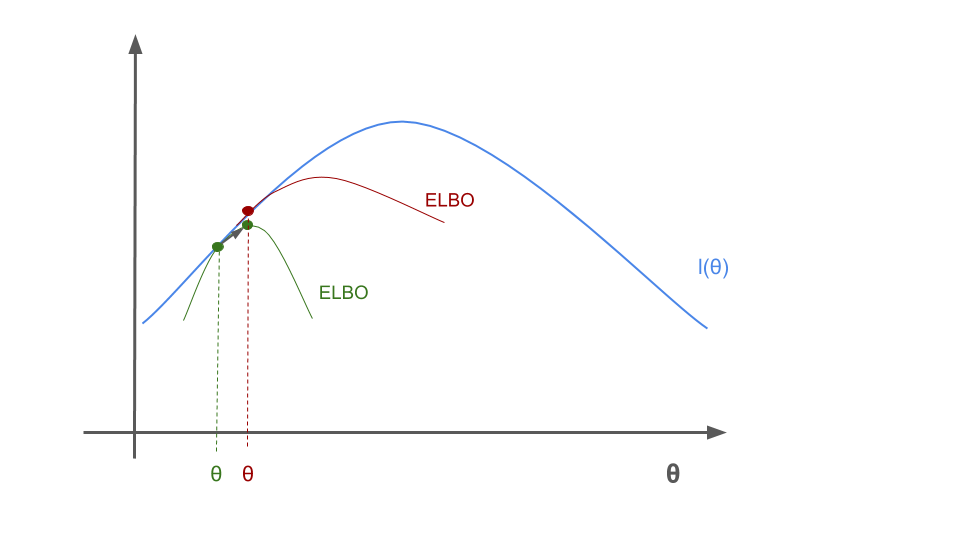
This seems all pretty abstract, lets have a look at a visualization of what happens for a simple case. First we draw the lower ELBO bound.

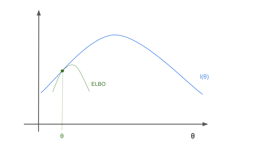
The we maximize \(\theta\) for the green ELBO bound.

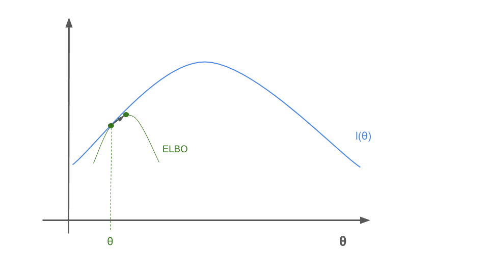
When we update \(Q\) then this gives us a new ELBO bound in red, which intersects at the same \(\theta\) value but improves the bound.

We maximize the new ELBO bound again

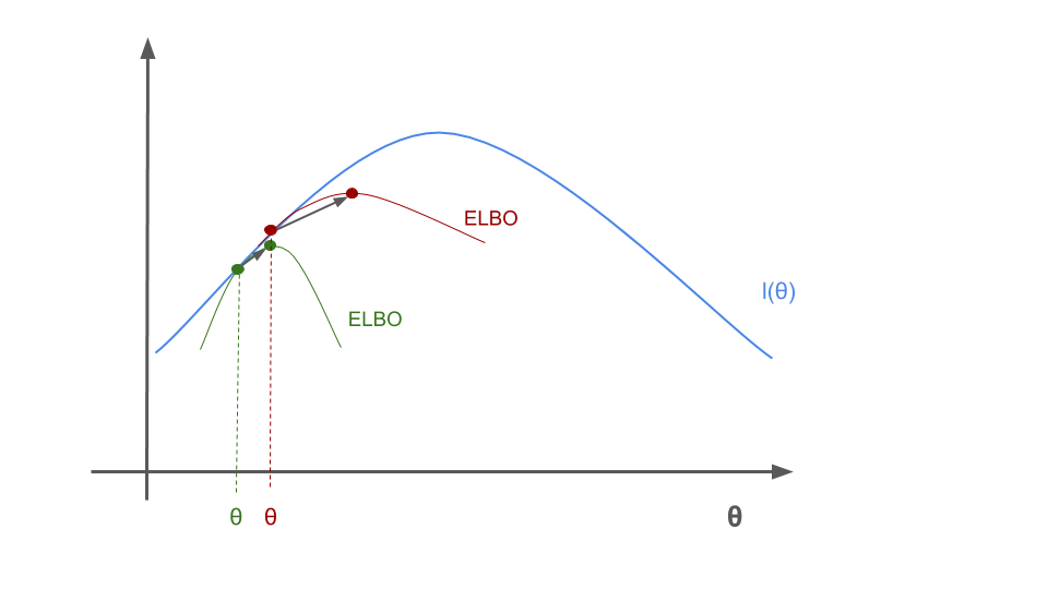
The process continues until convergence is reached. Note that this is a highly idealized example, we in reality we might optimize into a local optima for the likelihood.

The Case for Arbitrary Data

So far we were ignoring the full training set of \(n\) examples of data \(\lbrace x_1, \dotsc, x_n \rbrace\). The optimal choice for \(Q\) depended on the particular example \(x\) as we had \(Q(z) = p_{\theta}(z \mid x)\). The straightforward thing to do is to introduce \(n\) distributions \(Q_1, \dotsc, Q_n\), one for each example \(x_i\). Then for each \(x_i\) we can build the evidence lower bound:

\[\log(p_{\theta}(x_i)) \geq \text{ELBO}_{Q_i, \theta}(x_i) = \sum_{z_i} Q_i(z_i) \log \bigg(\frac{p_{\theta}(x_i,z_i)}{Q_i(z_i)}\bigg)\]

To obtain a lower bound for the likelihood function \(l(\theta)\) we sum over all the examples

\[\begin{align*} l(\theta) &\geq \sum_{i=1}^n \text{ELBO}_{Q_i, \theta}(x_i) \\ &= \sum_{i=1}^n \sum_{z_i} Q_i(z_i) \log \bigg(\frac{p_{\theta}(x_i,z_i)}{Q_i(z_i)}\bigg) \end{align*}\]

This gives a lower bound for any set of distributions \(Q_1, \dotsc, Q_n\) and as in the single data point case, to achieve equality we need

\[Q_i(z_i) = p_{\theta}(z_i \mid x_i)\]

For this choice of \(Q_i\)’s the inequality above gives a lower-bound on the log likelihood \(l\) that we are trying to maximize. This leads us to the general version of the EM algorithm. Repeat until convergence:

1. E-step

   For each \(i\) set

   \[Q_i(z_i) := p_{\theta}(z_i \mid x_i)\]

2. M-step

   Set

   \[\begin{align*} \theta &:= \text{arg} \max_{\theta} \sum_{i=1}^n \text{ELBO}_{Q_i, \theta}(x_i) \\ &= \text{arg} \max_{\theta} \sum_{i=1}^n \sum_{z_i} Q_i(z_i) \log \bigg(\frac{p_{\theta}(x_i,z_i)}{Q_i(z_i)}\bigg) \end{align*}\]

Monotonic Improvement

We saw in the images above why the algorithm intuitively improves for each iteration, now we have all the tools to proof it as well. Suppose we have parameters \(\theta_t\) and \(\theta_{t+1}\) from two successive iterations of EM. We need to prove that \(l(\theta_t) \leq l(\theta_{t+1})\). The key to show this result is the choice of \(Q_i\)’s. Remember we chose them in a way to make Jensen’s inequality tight, i.e. \(Q_i^t(z_i) := p_{\theta_t}(z_i \mid x_i)\). This gives us

\[l(\theta_t) = \sum_{i=1}^n \text{ELBO}_{Q_i^t, \theta_t}(x_i)\]

As the parameters \(\theta_{t+1}\) are obtained by taking the arg max of the right hand side, we get:

\[\begin{align*} l(\theta_{t+1}) &\geq \sum_{i=1}^n \text{ELBO}_{Q_i^t, \theta_{t+1}}(x_i) \\ &\geq \sum_{i=1}^n \text{ELBO}_{Q_i^t, \theta_t}(x_i) \\ &= l(\theta_t) \end{align*}\]

The first inequality follows from the fact that the ELBO is a lower bound for any choice of \(Q\) and \(\theta\), hence we can choose \(Q^t_i\) here. The above lines prove that EM causes the likelihood to converge monotonically. In practice we might not know when convergence is achieved, hence we would stop once the difference between successive iterations is small enough.

Conclusion

We saw three different algorithms, the \(k\)-means clustering, EM for mixtures of Gaussian and the general EM. At each step we removed assumptions to arrive at a general theory for EM algorithms. The properties remained similar throughout, we have a monotonic improvement from step to step, but no guarantee for convergence to a global optima.

Resources

A list of resources used to write this post, also useful for further reading:

• CS229 Syllabus - Contains all the resources for their excellent Machine Learning class
  • Lecture Notes 7a (pdf) - Contains the k-means clustering introduction
  • Lecture Notes 7b (pdf) - Contains the mixtures of Gaussians and the EM for the special case
  • Lecture Notes 8 (pdf) - Contains the general EM algorithm, revisits the Gaussian case and an introduction to variational inference

• [Lecture 14 - Expectation-Maximization Algorithms

  Stanford CS229: Machine Learning (Autumn 2018)](https://www.youtube.com/watch?v=rVfZHWTwXSA&list=PLoROMvodv4rMiGQp3WXShtMGgzqpfVfbU&index=14&ab_channel=stanfordonline) - for a lecture by Andrew Ng on k-means and Gaussian mixtures, plus an EM introduction

• [Lecture 15 - EM Algorithm & Factor Analysis

  Stanford CS229: Machine Learning (Autumn 2018)](https://www.youtube.com/watch?v=tw6cmL5STuY&list=PLoROMvodv4rMiGQp3WXShtMGgzqpfVfbU&index=15&ab_channel=stanfordonline) - for the general EM case and Factor Analysis

• Convex function - Wikipedia
• Concave function - Wikipedia
• Jensen’s inequality - Wikipedia

Comments

I would be happy to hear about any mistakes or inconsistencies in my post. Other suggestions are of course also welcome. You can either write a comment below or find my email address on the about page.