This post does a quick review of how Proximal Policy Optimization (PPO) and Direct Preference Optimization (DPO) work, and what their relationship to Reinforcement Learning from Human Feedback (RLHF) is. Especially RLHF has become popular over the past two years for fine-tuning networks beyond simple SFT. This phase is often called alignment, where we train a model to follow human preferences in a wide variety of tasks.

Unlike in classification or regression, the model can not simply learn one correct answer during RLHF. Simply because it does not exist for many tasks that LLM have to do (ex: “Give me a recipe for cooking that has chicken”).

Basic Concepts and Notation

Before we start, let us quickly repeat some basic concepts and their notation. Readers familiar with the topic may skip this section.

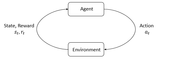
• Reinforcement Learning: In reinforcement learning an agent is taking actions \(a_t\) in an environment in state \(s_t\) and getting rewards \(r_t\).

• Policy: A rule used by an agent to decide what actions to take, if it is stochastic it is denoted by \(\pi\). It samples actions \(a_t\) from states \(s_t\): \(a_t \sim \pi( \cdot \mid s_t)\).

• Parametrized Policy: In deep RL we deal with parameterized policies, where the parameters are denoted by \(\theta\). Hence we write \(a_t \sim \pi_{\theta}(\cdot \mid s_t)\).

• On-Policy Value Function: \(V^{\pi}(s)\), which gives the expected return if you start in state \(s\) and always act according to policy \(\pi\):

• On-Policy Action-Value Function: \(Q^{\pi}(s,a)\), which gives the expected return if you start in state \(s\), take an arbitrary action \(a\) (not necessarily from the policy \(\pi\)), and then afterwards act according to policy \(\pi\):

• Advantage Function: The advantage function \(A^{\pi}(s,a)\) corresponding to a policy \(\pi\) describes how much better it is to take a specific action \(a\) in state \(s\), over randomly selecting an action according to \(\pi(\cdot \mid s)\). The advantage function is defined by:

• Kullback-Leibler Divergence: The KL-divergence of two probability distributions \(p\) and \(q\) is defined as

Often we consider \(p\) to be the true distribution and \(q\) the approximation or model output. Then the KL-divergence would give us a measure of how much information is lost when we approximate \(p\) with \(q\).

Reinforcement Learning from Human Feedback

Why do we need RLHF? Because LLMs are pre-trained on a large corpus of text (usually the entire internet) which contain a lot of mixed quality content and commonly held misbeliefs. In this phase of the training we want to bias the model towards higher quality output, not the median quality of a text on the internet. RLHF is also useful for cases where there is often no single right answer, we only give vague directions towards a better formulated response.

How does a typical RLHF training pipeline for LLMs look today?

1. Supervised fine-tuning: of a pre-trained LLM on high quality data for the tasks of interest.
2. Preference Rating: the SFT model is prompted with prompts \(x\) to produce pairs of answers \((y_1, y_2) \sim \pi^{SFT}(\cdot \mid x)\). These pairs are presented to human raters which will express preference for one answer over the other \(y_w \succ y_l \mid x\) where \(y_w\) and \(y_l\) denote the preferred and the dispreferred completion of the prompt \(x\).
3. Reward Modeling: The preferences are assumed to be generated by a reward model \(r^*(y, x)\) which we do not have access to. One way to model it is using the Bradley-Terry (BT) model, it stipulates that the human preference distribution \(p^*\) can be written as: \(p^*(y_1 \succ y_2 \mid x) = \frac{\exp(r^*(x, y_1))}{\exp(r^*(x, y_1)) + \exp(r^*(x, y_2))}\) We can parametrize the reward model as \(r_{\phi}(x,y)\) and estimate the parameters via maximum likelihood. Framing the problem as binary classification we can optimize the negative log-likelihood loss for data \(D\): \(L_R(r_{\phi}) = -E_{(x, y_w, y_l) \sim D} \bigg [ \log \sigma \Big(r_{\phi}(x,y_w) - r_{\phi}(x, y_l)\Big) \bigg]\)

with \(\sigma\) as the logistic function and the reward model \(r_{\phi}(x,y)\) initialized from the SFT model \(\pi^{SFT}(\cdot \mid x)\).

1. RL Fine-Tuning Phase: The learned reward model from step 3 is used to provide feedback to the language model. Because the loss is not differentiable for language tasks we use an reinforcement learning approach such as PPO, which we will see in depth in the next chapter.

The process of RLHF optimization is shown on the left.

PPO is used to finetune the baseline LLM based on rewards by the reward model. PPO is designed to be more stable and efficient than traditional policy gradient methods.

DPO is an alternative to use PPO within RLHF. It simplifies the fine-tuning process by directly optimizing the LLM based on the human ratings, without training a reward model. This works by reformulating the RL problem into a simpler classification problem, simplifying the training process.

Proximal Policy Optimization

This section is an overview of the 2017 paper from OpenAI called Proximal Policy Optimization Algorithms. This is pre-LLM hype, so the context for this paper is playing games.

Background

Policy Gradient Methods

We compute an estimator of the policy gradient and plug it into a stochastic gradient ascent algorithm. A commonly used gradient estimator is

The hats over \(g\) and \(E\) denote that we empirically estimate the quantities over a batch of samples. Typically alternating between sampling and optimization. In this case the gradient estimate \(\hat{g}\) is obtained by differentiating the loss function:

Trust Region Methods

Unconstrained optimization is problematic for large updates and can derail the training. Trust region methods try to mitigate this by only updating within a small trusted region where we believe that the approximation of the objective function is reasonably accurate. How do we define the trusted region? By ensuring that the KL-Divergence between the original and the updated policy stays small.

A typical method is Trust Region Policy Optimization (TRPO) which is a constrained optimization:

The theory behind TRPO suggests using a KL penalty and optimizing

instead. The choice of \(\beta\) is tricky and changes with every task.

Clipped Surrogate Objective

Let \(r_t(\theta)\) denote the probability ratio \(r_t (\theta) = \frac{\pi_{\theta} (a_t \mid s_t)}{ \pi_{\theta old}(a_t \mid s_t)}\). It follows that \(r(\theta_{old}) = 1\).

TRPO maximizes a “surrogate” objective

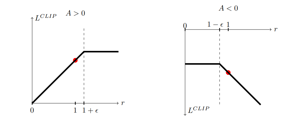
where CPI refers to Conservative Policy Iteration. Again this would have issues for large policy updates, which can be mitigated by clipping values of \(r_t(\theta) \hat{A_t}\) that move too far away from 1.

where \(\epsilon > 0\) is a hyperparameter. Empirically \(\epsilon = 0.2\) has been found to work well. What is the motivation behind this change?

There are two terms inside the min:

• First: \(r_t(\theta) \hat{A_t}\) is the \(L^{CPI}\)
• Second: \(\text{clip}(r_t(\theta), 1- \epsilon, 1+\epsilon) \hat{A_t}\) clips the probability ratio, i.e. it ensures that \(r_t(\theta) \in [1- \epsilon, 1+\epsilon]\).

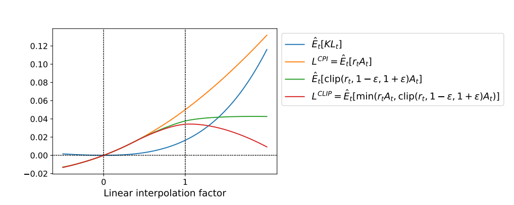
The minimum between the two terms ensures we take the lower bound (pessimistic estimate).

The figure above shows us how \(L^{\text{CLIP}}\) is a lower bound on \(L^{\text{CPI}}\).

PPO Algorithm

Most techniques for computing variance-reduced advantage function estimators make use of a learned state-value function \(V(s)\). If we are using a NN that shares parameters between the policy and value function, the loss function must use error terms for both tasks. Additionally the objective can be improved by adding an entropy bonus to ensure sufficient exploration. Combining these three terms gives:

where \(c_1, c_2\) are coefficients, \(S\) denotes an entropy bonus and \(L_t^{\text{VF}}\) is a squared-error loss:

Because the paper was written for environments with longer episodes in mind, we would usually run the policy for \(T\) timesteps (which is shorter than the episode length). In the case of RLHF we usually have \(T = 1 = \text{episode length}\).

The full PPO algorithm is then

for iteration=1, 2, . . . do 
  for actor=1, 2, . . . , N do 
    Run policy πθold in environment for T timesteps  
    Compute advantage estimates A_1, . . . , A_T
  end for
  Optimize surrogate L wrt θ, with K epochs and minibatch size M ≤ N T  
  θ_old ← θ 
end for

Direct Preference Optimization

The goal of DPO is to replace the RLHF process that includes PPO by something simpler that does not require a reward model. This approach leverages a particular choice of reward model parametrization to enable the extraction of the optimal policy in closed form, without an RL training loop.

The key insight is to replace the loss function over reward functions with a loss function over policies. The policy network will represent both the language model and the implicit reward.

Deriving the DPO objective

We start from the same RL objective as prior work under a general reward function \(r\)

where \(\beta\) is a parameter controlling the deviation from the reference policy \(\pi_{\text{ref}}\).

We can show that the optimal solution to the equation above has the form

for the partition function \(Z(x)\) defined as

Estimating this is impractical because we need to sum over all the possible answers in \(\Sigma_y\) for each question \(x\). However we can rearrange the equation for \(\pi_r(y \mid x)\) to express the reward function in terms of its corresponding optimal policy \(\pi_r\), the reference policy \(\pi_{ref}\) and the unknown partition function \(Z(\cdot)\).

Now we can apply this reparametrization to the ground-truth reward \(r^*\) and corresponding optimal model \(\pi^*\). The Bradley-Terry model only depends on the difference of rewards between two completions

We can now substitute the result from the derivation for \(r(x,y)\) into this equation to cancel out the partition function:

This is all under assumption of the Bradley-Terry model, the paper also derives results for more general models.

Now that we have the probability of human preference data in terms of the optimal policy rather than the reward model, we can formulate a maximum likelihood objective for a parametrized policy \(\pi_{\theta}\). The policy objective becomes:

What does the DPO update do?

To understand DPO better it is useful to take a look at the gradient of the loss function \(L_{DPO}\). The gradient w.r.t. the parameters \(\theta\) can be written as:

There are three different components in this loss:

1. \(\sigma \big(\hat{r}_{\theta}(x, y_l) - \hat{r}_{\theta}(x, y_w)\big)\) - higher weight when reward estimate is wrong.
2. \(\nabla_{\theta}\log \pi(y_w \mid x)\) - increase of likelihood of \(y_w\).
3. \(\nabla_{\theta} \log \pi(y_l \mid x)\) - decrease likelihood of \(y_l\).

DPO Algorithm

The DPO pipeline is as follows:

1. Sample completions \(y_1, y_2 \sim \pi_{\text{ref}}(\cdot \mid x)\) for every prompt \(x\) and label with humans to create preferences.
2. Optimize the language model \(\pi_{\theta}\) to minimize \(L_{DPO}\) for the given \(\pi_{\text{ref}}\), \(D\) and \(\beta\).

We would initialize \(\pi_{\text{ref}}\) as \(\pi_{SFT}\).

Conclusion

We have seen two different approaches to align models with human preferences. Whereas PPO is more general than DPO, it is also much harder to implement because it requires an extra training stage.

There is some evidence (see the paper “Unpacking DPO and PPO: Disentangling Best Practices for Learning from Preference Feedback”) that PPO leads to slightly higher quality results than DPO.

Final Thoughts

Some follow up questions and remarks for my future self or experts in this field:

• In PPO, how powerful should the reward model be? Can we gain a lot by having a large reward model and guide a smaller model? Is this problem similar to distillation?
• Do we lose any information when we train a reward model as opposed to directly using the human preference data? The paper suggests not but I’m not convinced by single digit improvements. I’ve generally found it preferable to directly optimize for whatever the final goal is, additional steps tend to dilute the signal.
• The paper comparing PPO and DPO suggests a slight advantage for PPO, but the PPO training process is much more involved. If we invested the same amount of time/effort/compute into improving the data, would we get better results for DPO?
• Both approaches still seem bounded by human performance, these approaches are unlikely to yield superhuman performance in a task (unlike AlphaZero).

References

A list of resources used to write this post, also useful for further reading:

• Proximal Policy Optimization Algorithms - John Schulman, Filip Wolski, Prafulla Dhariwal, Alec Radford, Oleg Klimov for the original DPO paper by OpenAI.

• Direct Preference Optimization: Your Language Model is Secretly a Reward Model - Rafael Rafailov, Archit Sharma, Eric Mitchell, Stefano Ermon, Christopher D. Manning, Chelsea Finn for the DPO paper by Stanford.
• Unpacking DPO and PPO: Disentangling Best Practices for Learning from Preference Feedback - Hamish Ivison, Yizhong Wang, Jiacheng Liu, Zeqiu Wu, Valentina Pyatkin, Nathan Lambert, Noah A. Smith, Yejin Choi, Hannaneh Hajishirzi for a paper that compares DPO and PPO on different tasks.
• Preference fine-tuning API by OpenAI for an example of an FT API.
• Introduction to RL by OpenAI Spinning UP.

Comments

I would be happy to hear about any mistakes or inconsistencies in my post. Other suggestions are of course also welcome. You can either write a comment below or find my email address on the about page.