When looking at a Deep Learning related project or paper, there are four fundamental parts for me: data, network architecture, optimization method and loss function. As the title suggests, here will focus on the last part. Loss functions are deeply tied to the task one is trying to solve, and are often used as measures of progress during training. In this post series we are going to see where they come from and why we using the ones we do. This first part will cover losses for the tasks of regression and classification.
Basic Concepts and Notation
Before we start, let us quickly repeat some basic concepts and their notation. Readers familiar with the topic may skip this section. This is not meant to be an introduction to probability theory or other mathematical concepts, only a quick refresh of what we will need later on.
-
Definition: If a term on the left hand side of the equation is defined as as the right hand side term, then \(:=\) will be used. This is similar to setting a variable in programming. As an example we can set \(g(x)\) to be \(x^2\) by writing \(g(x) := x^2\). In mathematics, when writing simply \(=\) means that the left side implies the right (denoted by \(\Rightarrow\)) and right side the left (denoted by \(\Leftarrow\)) at the same time.
-
Logarithm: \(\log : (0,\infty) \longrightarrow (-\infty, \infty)\). One of the basic function in calculus, known as the inverse of the exponential function \(x = \exp(\log(x))\). It has some properties which we will need later on:
- \(\log(xy) = \log(x) + \log(y)\) and \(\log\big(\frac{x}{y}\big) = \log(x) - log(y)\)
- For two bases \(b, k\), we have that \(\log_b(x) = \frac{\log_k(x)}{\log_k(b)} = C \cdot log_k(x)\) where \(C = \frac{1}{\log_k(b)}\) is a constant because it does not depend on \(x\). This means that a change of basis in the log is only a multiplication by a constant.
- If not mentioned otherwise, we will assume that \(b=e\), the natural logarithm.
- It is always useful to have an idea of how the plot of \(\log(x)\) looks like.
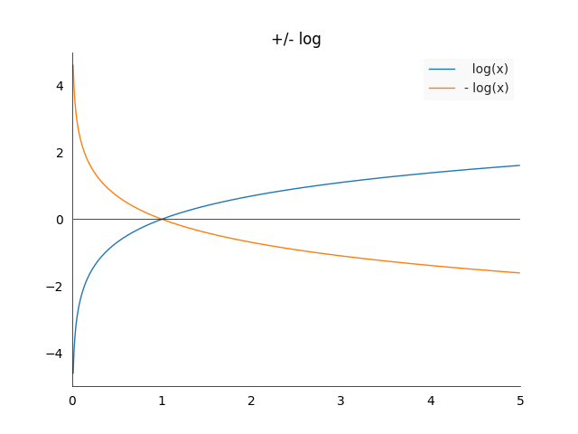 There are three cases which are worth noting:
- Log goes to minus infinity when approaching zero: \(\lim_{x \longrightarrow 0 } \log(x) = -\infty\)
- \(1\) is the only value for which log is equal to zero: \(\log(1) = 0\)
- Even if the graph looks like its flattening, it does actually go to infinity:\(\lim_{x \longrightarrow \infty} \log(x) = \infty\)
- Sigmoid: \(\sigma : (-\infty,\infty) \longrightarrow (0,1)\), is defined as \(\sigma(x) := \frac{1}{1+\exp(-x)} = \frac{\exp(x)}{1+\exp(x)}\). It has the property that it maps any value to the open interval \((0,1)\), which is very useful if we want to extract a probability from a model.
- The plot looks as follows:
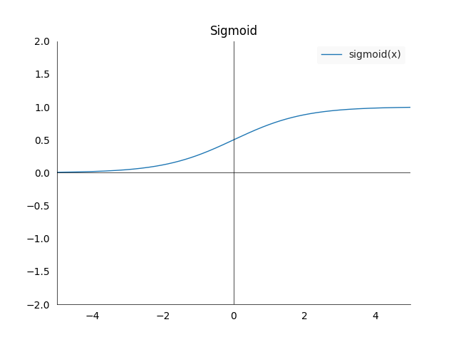
- Again three cases worth noting:
- The left limit is 0: \(\sigma(x)_{x \longrightarrow -\infty } = 0\)
- The right limit is 1: \(\sigma(x)_{x \longrightarrow \infty } = 1\)
- At zero we are in the middle of the range: \(\sigma(0) = 0.5\)
- The derivative of the sigmoid is \(\frac{\partial \sigma(x)}{\partial x} = \sigma(x) (1-\sigma(x))\)
- The plot looks as follows:
-
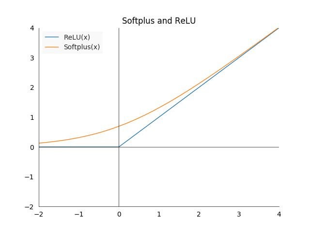
Softplus: \(\zeta : (-\infty,\infty) \longrightarrow (0,\infty)\) is defined as \(\zeta(x) := \log(1+\exp(x))\) the name comes from its close relationship with the function \(x^+ = \max(0,x)\), which deep learning practitioners know as rectified linear unit (ReLU). It is a softer version of \(x^+\) which becomes apparent when we draw them. It will frequently show up when we manipulate sigmoid functions in connection with Maximum Likelihood.
- This plot shows the difference between softplus and ReLU
- Some other noteworthy properties:
- The log sigmoid is softplus: \(-\log(\sigma(x)) = - \zeta(-x)\)
- The derivative of softplus is sigmoid: \(\frac{\partial \zeta(x)}{\partial x} = \frac{\exp(x)}{1+\exp(x)} = \sigma(x)\)
- This plot shows the difference between softplus and ReLU
-
Random Variable: A variable whose values depend on the outcomes of a random phenomenon, we usually denote it by \(X\) (upper case) and an outcome by \(x\) (lower case). An example would be a random variable X which represents a coin throw, it can take value zero for head or one for tail.
-
Probability Distribution: A function \(p\) associated with a random variable \(X\), it will tell us how likely an outcome \(x \in X\) is. In the case of a fair coin, we will have
\[P(X=0) = p_X(0) = p_X(1) = P(X=1) = \frac{1}{2}\]We usually omit the subscript \(p_X\) and only write \(p\) for simplicity. If we have an unnormalized probability distribution we will denote it with a hat: \(\hat{P}\). An unnormalized probability distribution does not need to sum up (in the discrete case) or integrate (continuous case) to one.
-
Expectation: For a random variable \(X\) the expectation is defined as
\[E(X) := \sum_{x \in X} p(x) x\]A weighted average of all the outcomes of a random variable (weighted by the probability). The expectation of the coin throw example is \(E(X) = 0 \cdot p(0) + 1 \cdot p(1) = 0 \cdot \frac{1}{2} + 1 \cdot \frac{1}{2} = \frac{1}{2}\).
-
(Strictly) Increasing transformation: a function \(f : \mathbb{R} \longrightarrow \mathbb{R}\) is a (strictly) increasing transformation if for all \(x, y \in \mathbb{R}\) with \(x \leq y\) (\(x < y\)) we have that \(f(x) \leq f(y)\) (\(f(x) < f(y)\)). These transformations have the property that we can apply them without changing the result whenever we care only about the ordering of elements, for example when minimizing a function.
-
Maximum Likelihood Estimation: For a probability distribution \(p_\theta\) with parameter \(\theta\) and data \(\lbrace x_1, \dotsc, x_n \rbrace\) we can estimate \(\theta\) by maximizing the probability over the data:
\[\theta = \text{argmax}_{\theta} p_{\theta}(x) = \prod_{i=1}^n p_{\theta}(x_i)\]This is called maximum likelihood estimation. Often it is more convenient to maximize the log likelihood instead, and because the log is a strictly increasing transformation the result will not change. The log transformation has the additional benefit that the product becomes a sum:
\[\theta = \text{argmax}_{\theta} \log(p_{\theta}(x)) = \sum_{i=1}^n \log(p_{\theta}(x_i))\]Which is beneficial when doing numerical optimization.
Notions of Distance
Distance
At the very bottom of loss functions are how we measure distances. In our daily life we switch between different measures of distance effortlessly. For example one could ask how far away are you from the next airport? You might measure this in time it takes to drive there, or the distance to the location in kilometers (or miles). If you chose to measure it in the latter way, you are most likely using Euclidean distance, but more on this later. In Mathematics there is a more general notion of distance on a set \(X\) (\(X\) could be anything, numbers, apples, oranges, mathematical objects). A distance \(d\) on the set \(X\) is a function
\[d : X \times X \longrightarrow \mathbb{R}\]such that
\[\begin{align*} 1. \; d(x,y) &\geq 0 & \forall x,y \in X\\ 2. \; d(x,y) &= 0 \Leftrightarrow x = y & \forall x,y \in X\\ 3. \; d(x,y) &= d(y,x) & \forall x,y \in X \\ 4. \; d(x,y) &\leq d(x,z) + d(z,y) & \forall x,y,z \in X \end{align*}\]These four conditions have straightforward interpretations. The first one tells us that a distance can never be negative. The second one says if the distance between two elements is zero, then they must be the same. The third one is symmetry, going from A to B is the same as going from B to A. The last one is called the triangle inequality, it can never be faster to go from A to C to B than going from A to B directly.
Euclidean Distance
The most well known example of a distance would be the Euclidean distance. In its general form the Euclidean distance between two n-dimensional real vectors \(x\) and \(y\), \(x,y \in \mathbb{R}^n\), is defined as follows:
\[d_E(x,y) := \sqrt{\sum_{i=1}^{n} (x_i - y_i)^2 }\]It is also often called the L2 norm, and denoted by \(\mid\mid \cdot \mid\mid_2\). In the two dimensional case this reduces to well known formula for calculating the hypotenuse of a triangle:
\[d_E(x,y) = \sqrt{(x_1 - y_1)^2 + (x_2-y_2)^2}\]L2 Norm and Linear Regression
The L2 norm is also widely used in machine learning, for example in linear regression. Remember that in linear regression we have a data matrix \(X \in \mathbb{R}^{n \times m}\) (\(n\) entries for \(m\) different variables), \(n\) labels or targets \(y \in \mathbb{R}^n\) and a parameter vector \(\beta \in \mathbb{R}^m\) which we are trying to fit such that \(y = X \beta\). However once we have \(n > m\), or more data than variables, there is no unique solution anymore. Hence we try to get as “as close as possible” to that state. And how do we measure closeness? By the squared L2 norm/Euclidean distance! We try to minimize
\[d_E(X\beta, y)^2 = \: \mid \mid X \beta - y\mid \mid^2_2\]Notice that we are trying to minimize the square of the Euclidean distance, this will not change the minimization result because it is a strictly increasing transformation. This distance measure has the advantage that we can easily calculate the optimal values for \(\beta\) by taking the partial derivative with respect to \(\beta\)
\[\begin{align*} \frac{\partial d_E(X \beta, y)^2}{\partial \beta} &= \frac{\partial((X\beta y)^T(X\beta -y))}{\partial \beta}\\ &= \frac{\partial(\beta^TX^TX\beta - \beta^TX^Ty-y^TX\beta -y^Ty)}{\partial \beta} \\ &= \frac{\partial \beta^TX^TX\beta}{\partial \beta} - \frac{\partial \beta^TX^Ty}{\partial \beta} - \frac{\partial y^TX\beta}{\partial \beta} -\frac{\partial y^Ty}{\partial \beta} \\ &= 2X^TX\beta -X^Ty -y^TX - 0 \\ &= 2X^TX\beta -2X^Ty \end{align*}\]To find the optimal we set the derivative with respect to \(\beta\) to zero and solve for \(\beta\) \(\begin{align*} 0 &= 2X^TX\beta -2X^Ty & \Leftrightarrow \\ 2X^Ty &= 2X^TX\beta & \Leftrightarrow \\ (X^TX)^{-1}X^Ty &= \beta \end{align*}\)
Where the last line gives us a unique solution for \(\beta\), which of course only applies if the assumptions of linear regression are true.
The Euclidean distance works well for measuring the distance between vectors, but what if we want to measure the distance between probability distributions? This is what lies at the heart of classification. Here the labels are one-hot encoded vectors and the model output is a vector of probabilities. Note that a one-hot encoded vector is just a probability distribution where the mass is concentrated in a single class. Hence the need for a way to compare probabilities.
Divergence
This is what a divergence function does, it gives us a sense of distance between two distributions. It is not exactly a distance because it is weaker, in the sense that a divergence measure has to fulfill less strict criteria. If \(S\) is the space of all probability functions on a random variable \(X\), then a divergence on \(S\) is a function
\[D : S \times S \longrightarrow \mathbb{R}\]satisfying
\[\begin{align*} 1. \; D(p \mid\mid q) & \geq 0 & \forall p,q \in S\\ 2. \; D(p \mid\mid q) &= 0 \Leftrightarrow p = q & \forall p,q \in S \end{align*}\]We can see that we only require the first two conditions from the definition of a distance. This means that in general a divergence will not be symmetric, i.e. \(D(p \mid\mid q) \neq D(q \mid\mid p)\) and the triangle inequality will not hold. Let us have a look at a concrete example of a divergence which is widely used in statistics and machine learning.
Kullback-Leibler Divergence
The Kullback-Leibler divergence or KL-divergence is often used to compare two probability distributions \(p,q \in S\). Remember that \(p, q\) are defined on the random variable \(X\), and \(x \in X\) denotes a single event. For example if \(X\) is all the possible outcomes of a dice throw, then \(x\) could be the event that 6 ends up on top. A probability distribution \(p\) assigns a probability to each event in \(x \in X\), in the example of a fair dice we would have \(p(x)= \frac{1}{6} \quad \forall x \in \lbrace 1,2,3,4,5,6\rbrace\).
The KL-divergence of two probability distributions \(p\) and \(q\) is defined as
\[D_{KL}(p \mid\mid q) := \sum_{x \in X} p(x) \log\bigg(\frac{p(x)}{q(x)}\bigg) = - \sum_{x \in X} p(x) \log\bigg(\frac{q(x)}{p(x)}\bigg).\]In the third term we simply switched the order of \(p\) and \(q\) to take out a minus sign, this form of the KL-Divergence will show up later. Note that we can view the KL-divergence as the expectation of the log difference between \(p\) and \(q\). This is because of
\[\begin{align*} D_{KL}(p \mid\mid q) &= \sum_{x \in X} p(x) \log\bigg(\frac{p(x)}{q(x)}\bigg)\\ &= \sum_{x \in X} p(x) (\log(p(x)) - \log(q(x)) \\ &= E\big(\log(p(X)) - \log(q(X))\big) \end{align*}\]Often we consider \(p\) to be the true distribution and \(q\) the approximation or model output. Then the KL-divergence would give us a measure of how much information is lost when we approximate \(p\) with \(q\). We can minimize the divergence to find a \(q\) which is closer to \(p\). First, we need to take a small detour through information theory to arrive at a loss function for classification.
Entropy
The self-information of an event \(x \in X\) in a probability distribution \(p\) is defined as
\[I(x) = - \log(p(x))\]For a probability \(p\) distribution on a random variable \(X\), the entropy \(H\) of \(p\) is defined as
\[H_b(p) := -\sum_{x \in X} p(x) \log_b(p(x)) = E(I(X))\]where \(b\) is the base of the logarithm, it is used to choose the unit of information. If \(b=2\), then the unit of information is bits, for \(b=e\) the unit is nats. However changing the base will only rescale entropy, it will not change the order of different distributions, i.e. if \(H_2(p) > H_2(q)\) then \(H_e(p) > H_e(q)\) for two probability distributions \(p, q\).
The term on the right hand side shows an interpretation of the entropy, it can be seen as the expected amount of information from an event drawn from distribution \(p\). It allows us to quantify the uncertainty or information in a probability distribution. The entropy is maximal for a uniform distribution. Note that the entropy is defined on a single probability distribution and does not allow for a direct comparison, this will be the next step as we now have all the tools necessary to define cross-entropy.
Cross-Entropy
The cross-entropy between two probability distributions \(p\) an \(q\) is defined as
\[H(p,q) := H(p) + D_{KL}( p \mid \mid q)\]Cross-entropy is the sum of the entropy of the target variable and the penalty which we incur by approximating the true distribution \(p\) with the distribution \(q\). The terms can be simplified:
\[\begin{align*} H(p,q) &= H(p) + D_{KL}( p \mid \mid q) \\ &= -\sum_{x \in X} p(x) \log(p(x)) - \sum_{x \in X} p(x) \log\bigg(\frac{q(x)}{p(x)}\bigg) \\ &= -\sum_{x \in X} p(x) \log(p(x)) - \sum_{x \in X} p(x) \log(q(x)) + \sum_{x \in X} p(x)\log(p(x)) \\ &= - \sum_{x \in X} p(x) \log(q(x)) \end{align*}\]In words it is the information of events in \(q\) weighted by \(p\). How does cross-entropy compare to KL-divergence? In terms of information theory, KL-divergence is sometimes also called relative entropy, the term becomes more meaningful when we look a the following two statements:
- Cross-Entropy: Average number of total bits to represent an event from \(q\) instead of \(p\).
- Relative-Entropy: Average number of extra bits to represent an event from \(q\) instead of \(p\).
Moreover we can see that on the right hand side of the equation for cross-entropy, only the KL-divergence depends on \(q\), thus minimizing cross-entropy with respect to \(q\) is equivalent to minimizing the KL-divergence.
Loss functions for Classification
So far we have seen that cross-entropy or KL-divergence makes sense as a distance measure for probability distributions, but why don’t we use L2 or an entirely different measure? We will see that there are certain properties, intuitive and in connection with gradient descent, that make it a better choice than for example L2.
Intuitive Properties of Cross-Entropy
Let \(x_T \in \mathbb{R}\) and \(l_{x_T}: \mathbb{R} \longrightarrow [0,\infty)\) be a generic loss function for a target value \(x_t\). Note that this is similar to a distance function where we fix one input to be \(x_T\), i.e. \(l_{x_T}(x) = d(x_T, x)\). What kind of intuitive properties would we like our loss function to have?
- The loss for the target value should be zero: \(l_{x_T}(x_T) = 0\).
- The loss for any \(x\) not equal to \(x_T\) should be bigger than zero: \(x \in \mathbb{R}, x \neq x_T \quad \Rightarrow \quad l_{x_T}(x) > 0\).
- Monotonicity. For two values \(x_1, x_2 \in \mathbb{R}\) such that \(x_2\) is further away from true value \(x_T\) than \(x_1\), the loss should be bigger for \(x_2\): \(| x_2 - x_T | > | x_1 - x_T| \quad \Rightarrow \quad l_{x_T}(x_2) > l_{x_T}(x_1)\).
There are a lot of functions which satisfy these properties besides cross-entropy. For example the absolute \(l_{x_T}(x)=\mid x - x_T \mid\) or the quadratic \(l_{x_T}(x) = (x- x_T)^2\) loss do have that property. If we set \(x_T = 1\), we can plot them together for a simpler comparison:
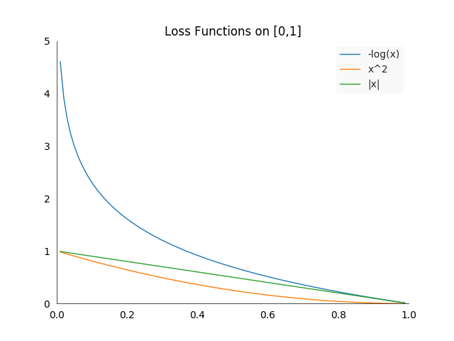
Notice that they are only plotted on the interval \([0,1]\), because that is what interests us for classification. Suppose we have an additional requirement which is a bit more fluffy: we would like to strongly punish confident but wrong predictions. This is where the \(-log(x)\) function excels. In theory, if you predict zero for a true label of one, your loss will be infinite, in reality our systems do not handle extremely large values well. Nevertheless, it gives superior feedback to most other loss functions.
Properties in Connection with Gradient Descent
To show the connection between cross-entropy and gradient descent, we will have to do once again a quick detour. Suppose we have a model \(f: \mathbb{R}^n \longrightarrow \mathbb{R}\), which takes an input vector \(x\) and outputs an arbitrary number \(y = f(x)\). For example the model could be a linear layer \(f(x) = x^Th + b\), or even a more complicated neural network. We want to do binary classification, i.e. differentiating between two different classes of input.
For the rest of this chapter to work, we will have to make the assumption that the response is monotone with respect to the input, that means if \(f(x) \longrightarrow \infty\) it is more confident that the class is one. And in the opposite direction if \(f(x) \longrightarrow -\infty\), it is more confident that the class is zero. Now we can create a decision boundary to decide which class to predict, for example if \(f(x) > 0\) we predict class one, otherwise zero. If the model is linear that would be called a linear classifier and the the rule a threshold function.
A binary classification task can be modeled by a Bernoulli variable \(Z \sim B(p)\). A Bernoulli random variable takes values in \(\lbrace 0, 1 \rbrace\), where \(P(Z=1) = p\) and \(P(Z=0) = 1-p\). Notice that there is only one parameter to estimate, hence it is sufficient to model \(P(Z=1 \mid x)\), the probability of the input \(x\) being of class one. For now our model returns values in \(\mathbb{R}\), hence we need to restrict it. A naive approach would be to extract the probability by using
\[P(Z=1 \mid x) = \max\big(0, \min(1, f(x))\big)\]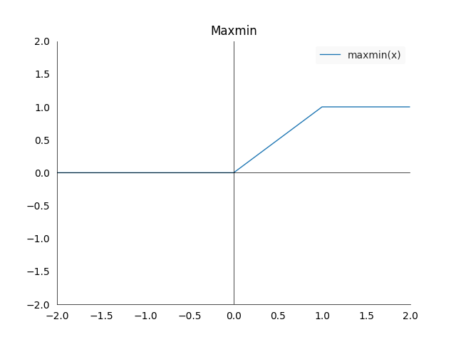
The problem with this approach is that the gradient would be zero outside of \([0,1]\). This means our model would not learn from any samples which lie outside of that interval.
A better approach can be deducted from the following reasoning. Remember we modeled our problem by a Bernoulli random variable \(Z\), which has probability distribution \(P(z)\), which we are trying to approximate. If we now assume that the unnormalized log probabilities \(\log( \hat{P}(z))\) are linear in \(y\) and \(z\), we can construct:
\[\begin{align*} \log( \hat{P}(z)) &= yz\\ \hat{P}(z) &= \exp(yz) \\ P(z) &= \frac{\exp(yz)}{\sum_{z^*=0}^1 \exp(yz^*)} \\ P(z) &= \sigma((2z-1)y) \end{align*}\]Remember that \(\sigma(x) = \frac{\exp(x)}{1+\exp(x)}\), \(z \in \lbrace 0,1 \rbrace\) and \(y \in \mathbb{R}\). The last term is slightly difficult to unpack. One way to do that is by a case distinction. Keep in mind that we assume that if the model output \(y\) is high, we want to predict one, and vice versa if the output is strongly negative we should predict zero:
- For \(z = 0\): We have that \(P(z) = P(0) = \sigma((0-1)y) = \sigma(-y) = \frac{\exp(-y)}{1+\exp(-y)}\).
-
\[\lim_{y \longrightarrow \infty} = \frac{\exp(-y)}{1+\exp(-y)} = 0\]
This means in the case that the true label is zero, and our model output \(y =f(x)\) goes towards \(\infty\), the probability of the label being zero is \(0\).
-
\[\lim_{y \longrightarrow -\infty} = \frac{\exp(-y)}{1+\exp(-y)} = 1\]
This means in the case that the true label is zero, and our model output \(y =f(x)\) goes towards \(-\infty\), the probability of the label being zero is \(1\).
-
\[\lim_{y \longrightarrow \infty} = \frac{\exp(-y)}{1+\exp(-y)} = 0\]
- For \(z = 1\): We have that \(P(z) = P(1) = \sigma((2-1)y) = \sigma(y) = \frac{\exp(y)}{1+\exp(y)}\)
-
\[\lim_{y \longrightarrow \infty} = \frac{\exp(y)}{1+\exp(y)} = 1\]
This means in the case that the true label is one, and our model output \(y =f(x)\) goes towards \(\infty\), the probability of the label being one is \(1\).
-
\[\lim_{y \longrightarrow -\infty} = \frac{\exp(y)}{1+\exp(y)} = 0\]
This means in the case that the true label is one, and our model output \(y =f(x)\) goes towards \(-\infty\), the probability of the label being one is \(0\).
-
\[\lim_{y \longrightarrow \infty} = \frac{\exp(y)}{1+\exp(y)} = 1\]
After this slightly tedious motivation we can now finally apply the cross-entropy loss to our model. In the case of two classes, with true class \(z\) and predicted probability \(p = \sigma((2z-1)y)\), it reduces to
\[l_z(p) = -z\log(p) - (1-z) \log(1-p)\]We need to estimate only the case \(P(z=1)\) for which the loss transforms to
\[\begin{align*} l_z(p) &= - \log(p) \\ &= -\log\big(\sigma((2z-1)y)\big) \\ &= -\log\bigg( \frac{1}{1+\exp(-(2z-1)y)}\bigg)\\ &= \zeta((1-2z)y) \end{align*}\]So our loss ends up being a softplus function, again due to the convoluted last term it is a bit hard to see what the actual behavior will be. Remember that the softplus function \(\zeta(x)\) is basically linear for \(x > 0\) and zero for \(x < 0\). This means
- For \(z=1\)
- If \(y \gg 0\) then \(\zeta(-y) \approx 0\) the model prediction is correct and we don’t want to change the model, the loss should be zero.
- If \(y \ll 0\) then \(\zeta(-y) \approx y\), our prediction was wrong, the more confident the model was the bigger the loss should be.
- For \(z=0\):
- If \(y \gg 0\) then \(\zeta(y) \approx y\), the model prediction is wrong, the more confident the model was the bigger the loss should be.
- If \(y \ll 0\) then \(\zeta(y) \approx 0\), the model prediction is correct and we do not want to change the model, the loss should be zero.
In both cases when the prediction is wrong, the derivative of the function approximates one, the loss function will not shrink the gradient no matter how wrong the prediction is.
Question: Do you see why adding a ReLu after the last layer is not great but does not have a large influence on classification performance?
What About a Different Loss Function?
Suppose we use a different loss function such as quadratic loss: \(l(x) = x^2\). Then our loss term becomes
\[l_z(p) = (z-p)^2 = \big(z - \sigma((2z-1)y)\big)^2\]To simplify the gradient calculation, we will replace the sigmoid term with \(\sigma(x)\), this will not change the point we are making.
\[\begin{align*} \frac{\partial l_z(p)}{\partial x} &= \frac{\partial (z-p)^2}{\partial x} \\ &= \frac{\partial (z-\sigma(x))^2}{\partial x}\\ &= 2 \frac{\partial (z-\sigma(x))}{\partial x}\\ &= 2 \frac{\partial \sigma(x)}{\partial x}\\ &= 2 \sigma(x)(1-\sigma(x)) \end{align*}\]Suppose that \(x \gg 0\), then sigma is in a extremely saturated region, the first sigma term will be almost one, but the second will be almost zero! This will shrink the gradient considerably, the model will be unable to learn. The same happens when \(x \ll 0\), then the first sigma term will be almost zero. These cases show that confident but wrong predictions will not be punished with a strong gradient, not a good property to have.
Generalizing to Multiple Classes
The previous example worked well for predicting two different classes, but what if we have \(n\) different classes? Before we modeled the process by a Bernoulli distribution and the model produced only a single output value to predict the log probability of class one, \(p = \log(\hat{P}(z = 1 \mid x))\). Now, we model the process by a multinomial distribution with only one trial, i.e. \(Z \sim \text{Multi}(t,p)\) where \(t=1\) and \(p \in \mathbb{R}^n\) is a vector containing probabilities. It has to have the properties \(p_i \in [0,1]\) and \(\sum_{i=1}^n p_i = 1\). Additionally we assume the model \(f\) produces an \(n\)-dimensional vector as output: \(y = f(x) \in \mathbb{R}^n\).
We can use a similar approach as in the binomial case and assume that the \(i\)-th output predicts log probabilities. Then we exponentiate and normalize to arrive at softmax
\[\begin{align*} \log\big(\hat{P}(z=i \mid x))\big) &= y_i \\ \hat{P}(z=i \mid x)) &= \exp(y_i) \\ P(z=i \mid x) &= \frac{\exp(y_i)}{\sum_{k=1}^n \exp(y_k)} \\ &= \text{softmax}(y)_i \\ &= s_i \qquad \qquad \qquad \forall i \in \lbrace 1, \dotsc,n \rbrace \end{align*}\]Notice that the softmax function does not change the dimension of the vector, it will stay \(n\) dimensional. However the vector \(s\) represents a probability distribution as indicated by the \(P\) without the hat. Similar as with the sigmoid, the softmax works well when using a cross-entropy loss function. The general version of the loss is
\[l_z(s) = -\sum_{i=1}^n \mathbb{1}_{i=z} \log(s_i)\]Where \(z\) is now a one-hot encoded vector with the true label being one and a zero everywhere else. The symbol \(\mathbb{1}_c\) stands for the indicator function, which is one when the condition \(c\) is true and zero otherwise. This means only one term of the sum will be non-zero and influence the loss. We can simplify the loss to see it decomposed into two terms
\[\begin{align*} -\log(s_i) &= -\log(\text{softmax}(y)_i) \\ &= -\log\Bigg(\frac{\exp(y_i)}{\sum_{k=1}^n \exp(y_k)}\Bigg) \\ &= -\log(\exp(y_i)) + \log\Bigg(\sum_{k=1}^n \exp(y_k)\Bigg) \\ &= - y_i + \log\Bigg(\sum_{k=1}^n \exp(y_k)\Bigg). \end{align*}\]Notice that the last term depends directly on the value of \(y_i\), our model output. Hence the loss function can not saturate and our optimization can always proceed. The left term \(y_i\) will always try to grow and the right term will be minimized.
We can approximate the sum on the right side by the biggest term of the sum: \(\sum_{k=1}^n \exp(y_k) \approx \exp(x_l)\), where \(x_l\) is the largest of the \(n\) terms. This is because the exponential function grows very fast and all other terms than the maximum will have an negligible influence on the sum. This tells us that the loss function will strongly penalize the most active incorrect prediction. However, if the biggest term in the sum is \(\exp(y_i)\), the same index as the true class, then the loss simplifies to \(\zeta(y_i)- y_i \approx 0\), it would be close to zero.
Like the sigmoid which saturates when the input value becomes extreme, the softmax function can saturate when the difference between the input values becomes large. This will lead to problems for all loss functions which do not invert the saturating property. As we saw above, cross-entropy does not have that issue.
Numerical Stability
Using exponentials can lead to large values, which can bring numerical systems to their limits. However there are some tricks which lets us use them safely. An interesting property of the softmax is that is invariant to the addition of constants, for \(c \in \mathbb{R}\) we have
\[\begin{align*} \text{softmax}(y+c)_i &= \frac{\exp(y_i+c)}{\sum_{k=1}^n \exp(y_k+c)} \\ &= \frac{\exp(y_i)\exp(c)}{\sum_{k=1}^n \exp(y_k)\exp(c)} \\ &= \frac{\exp(y_i)}{\sum_{k=1}^n \exp(y_k)} \\ &= \text{softmax}(y)_i. \end{align*}\]This can be used to create a numerically stable version of the softmax, where we subtract the largest value in vector \(y\) from all the terms.
\[\text{softmax}(y)_i = \text{softmax}\bigg(y-\max_k(y_k)\bigg)_i\]This does not apply to the sigmoid function, as it contains terms which are not exponentiated. However it can be written in two different forms:
\[\sigma(x) = \frac{1}{1+\exp(-x)} = \frac{\exp(x)}{1+\exp(x)}\]The first form is more suitable for large values \(x \gg 0\), while the second one is more suitable for extremely small values of \(x \ll 0\).
Conclusion
In the first part of this post we saw different notions of distance, for points in space and probability distributions. Later we saw what connects KL-divergence, entropy and cross-entropy. The second part focused on what makes cross-entropy well suited for classification in combination with gradient descent.
References
A list of resources used to write this post, also useful for further reading:
- Deep Learning Book by Goodfellow, Bengio and Courville
- Softmax Wikipedia
- Sigmoid Wikipedia
- Loss functions for classification Wikipedia
- Entropy Wikipedia, for definition and examples
- Cross-Entropy Wikipedia, for relationship to minimization, KL-divergence and log-likelihood
- Kullback-Leibler Divergence Wikipedia, for relationship to Cross-Entropy and interpretations
- Divergence in Statistics Wikipedia, for definition and properties of divergence
- Rectifier Wikipedia, for softplus and ReLU
- Cross-Entropy for Machine Learning Blog post, for various relationships between entropy and cross-entropy
- Loss functions for training deep learning neural networks Blog post, for discussion on various losses
Comments
I would be happy to hear about any mistakes or inconsistencies in my post. Other suggestions are of course also welcome. You can either write a comment below or find my email address on the about page.