In the past few years, LLMs have been revolutionizing how we interact with computers. There have been consequences for computer vision as well, in this post we are going to take a look on how vision was impacted by the new opportunities LLMs have brought us. More specifically, we are going to discover how we went to pre-training on fixed categories to all the images on the internet.

This blog post will mostly focus on how the process of pre-training for vision models has changed, we will not look at the architecture of the models itself (CNNs vs ViT).

Basic Concepts and Notation

Before we start, let us quickly repeat some basic concepts and their notation. Readers familiar with the topic may skip this section.

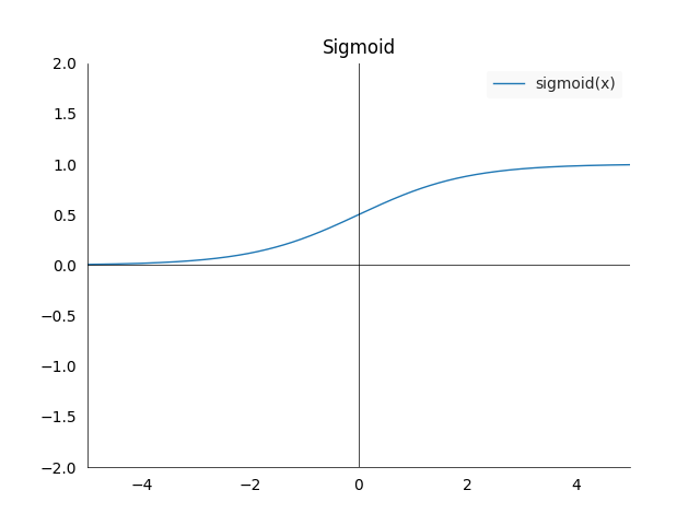
Sigmoid: σ:(−∞,∞)⟶(0,1), is defined as σ(x):=11+exp(−x)=exp(x)1+exp(x). It has the property that it maps any value to the open interval (0,1), which is very useful if we want to extract a probability from a model.
- The plot looks as follows:
- Again three cases worth noting:
  - The left limit is 0: $\sigma(x)_{x \longrightarrow -\infty } = 0$
  - The right limit is 1: $\sigma(x)_{x \longrightarrow \infty } = 1$
  - At zero we are in the middle of the limits: $\sigma(0) = 0.5$
- The derivative of the sigmoid is $\frac{\partial \sigma(x)}{\partial x} = \sigma(x) (1-\sigma(x))$
Dot product: The dot product between two vectors $\mathbf{a}, \mathbf{b} \in \mathbb{R}^n$ is defined as
$\mathbf{a} \cdot \mathbf{b} := \sum_{i=1}^n a_i b_i$

The dot product for non-zero vectors will be zero if the they are in a 90 degree angle.

Cosine similarity: The cosine similarity is the normalized dot product between to vectors $\mathbf{a}, \mathbf{b} \in \mathbb{R}^n$ :

$\cos(\theta) = \frac{a \cdot b}{\mid \mid a \mid \mid \cdot \mid \mid b \mid \mid}$

It measures the angle between two vectors and is independent of their magnitude.

Softmax: The basic softmax function is defined as:

$\text{softmax}(z)_i = \frac{e^{z_i}}{\sum_{j=1}^{N} e^{z_j}}$

here $z$ is a vector of scores and $N$ is the number of elements in $z$ .

Softmax trick: Large values for $z$ , $e^{z_i}$ can lead to numerical instability (overflow). To address this, we use the “softmax trick”:

$\text{softmax}(z)_i = \frac{e^{z_i - \max(z)}}{\sum_{j=1}^{N} e^{z_j - \max(z)}}$

where $\max(z)$ is the maximum value in the vector $z$ . This works because

Let $c = \max(z)$ . Then:

$\begin{align*} \text{softmax}(z)_i &= \frac{e^{z_i - c}}{\sum_{j=1}^{N} e^{z_j - c}} \\ &= \frac{e^{z_i} e^{-c}}{\sum_{j=1}^{N} e^{z_j} e^{-c}} \\ &= \frac{e^{-c} e^{z_i}}{e^{-c} \sum_{j=1}^{N} e^{z_j}} \\ &= \frac{e^{z_i}}{\sum_{j=1}^{N} e^{z_j}} \end{align*}$

Entropy: The self-information of an event $x \in X$ in a probability distribution $p$ is defined as

$I(x) = - \log(p(x))$

For a probability $p$ distribution on a random variable $X$ , the entropy $H$ of $p$ is defined as

$H_b(p) := -\sum_{x \in X} p(x) \log_b(p(x)) = E(I(X))$

where $b$ is the base of the logarithm, it is used to choose the unit of information.

Kullback-Leibler Divergence: The KL-divergence of two probability distributions $p$ and $q$ is defined as

$D_{KL}(p \mid\mid q) := \sum_{x \in X} p(x) \log\bigg(\frac{p(x)}{q(x)}\bigg) = - \sum_{x \in X} p(x) \log\bigg(\frac{q(x)}{p(x)}\bigg)$

Often we consider $p$ to be the true distribution and $q$ the approximation or model output. Then the KL-divergence would give us a measure of how much information is lost when we approximate $p$ with $q$ . If the KL divergence is zero, then the two distributions are equal.

Cross-Entropy: The cross-entropy between two probability distributions $p$ an $q$ is defined as

$H(p,q) := H(p) + D_{KL}( p \mid \mid q)$

Cross-entropy is the sum of the entropy of the target variable and the penalty which we incur by approximating the true distribution $p$ with the distribution $q$ . The terms can be simplified:

$\begin{align*} H(p,q) &= H(p) + D_{KL}( p \mid \mid q) \\ &= -\sum_{x \in X} p(x) \log(p(x)) - \sum_{x \in X} p(x) \log\bigg(\frac{q(x)}{p(x)}\bigg) \\ &= -\sum_{x \in X} p(x) \log(p(x)) - \sum_{x \in X} p(x) \log(q(x)) + \sum_{x \in X} p(x)\log(p(x)) \\ &= - \sum_{x \in X} p(x) \log(q(x)) \end{align*}$

Only the KL-divergence depends on $q$ , thus minimizing cross-entropy with respect to $q$ is equivalent to minimizing the KL-divergence.

Symmetric vs Asymmetric Cross-Entropy loss: Since the KL-divergence is asymmetric, the CE-loss is also asymetric. This means the penalty for false positive is different from the penalty for a false negative. It is more sensitive to errors predicting the true class. This can be problematic when dealing with noisy labels, the model may overfit to incorrect information.

The standard cross-entropy loss is given by:

$L_{CE}(y, \hat{y}) = - \sum_{i=1}^{C} y_i \log(\hat{y}_i)$

To create a symmetric cross-entropy loss, we can combine the standard cross-entropy with its reverse:

$L_{RCE}(\hat{y}, y) = - \sum_{i=1}^{C} \hat{y}_i \log(y_i)$

The symmetric cross-entropy loss, $L_{SCE}$ , can be defined as a combination of these two losses. A simple combination is the average:

$L_{SCE}(y, \hat{y}) = \frac{1}{2} \left[ L_{CE}(y, \hat{y}) + L_{RCE}(\hat{y}, y) \right]$

Substituting the definitions of $L_{CE}$ and $L_{RCE}$ , we get:

$L_{SCE}(y, \hat{y}) = -\frac{1}{2} \sum_{i=1}^{C} \left[ y_i \log(\hat{y}_i) + \hat{y}_i \log(y_i) \right]$

InfoNCE loss: Introduced by van der Oord et al in their paper Representation Learning with Contrastive Predictive Coding. We want to maximize the mutual information between two original signals $x$ and $c$ defined as

$I(x, c) = \sum_{x, c} p(x, c) \log \frac{p(x \mid c)}{p(x)}$

We want to model the density ratio of the signals as

$f(x_t, c_t) \propto \frac{p(x_t \mid c_t)}{p(x_t)}$

where $f$ is a model that is proportional to the true density, but does not have to integrate to 1. Given a set $X = \lbrace x_1, \dotsc, x_N \rbrace$ of $N$ random samples containing one positive sample from $p(x_t \mid c_t)$ and $N − 1$ negative samples from the ’proposal’ distribution $p(x_t)$ , we optimize

$L_{RCE}(x, c) = - E_X \bigg \lbrace \log \frac{f(x_t, c_t)}{\sum_{x_j \in X} f(x_j, c_t)} \bigg \rbrace$

This loss will result in $f(x_t, c_t)$ estimating the density ratio in the previous equation. For a proof see the paper. In other words, the InfoNCE loss encourages similar items to have similar embeddings and disimilar items to have different embeddings.

Contrastive Language Image Pretraining (CLIP) - Feb 2021

This paper from OpenAI in 2021 introduces a new way of combining vision and language that scales with unlabled data and goes from predicting fixed pre-defined categories to free from text. It enabled zero-shot transfer to new tasks that were competitive with a fully supervised baseline.

During that time, GPT-3 showed what was possible in language: pre-train with self-supervised objective on enough data with enough compute and the models became competitive on many tasks with little to no task-specific data. This showed that web-scale data could surpass high-quality crowd-labeled NLP datasets. In computer vision this was not yet standard.

One option to take advantage of web-scale data was to pre-train models on noisy labeled datasets with classification tasks. Typical datasets would be ImageNet or JFT-300M (Google internal). These pre-trained backbones were then fine tuned on task specific training sets. This is also the approach we used at places where I worked at time (2018-2021). However these pre-training approaches all used softmax losses to predict various categories. This limits the concepts that they learn to the specific categories in the pre-training sets and makes it harder to generalize in zero-shot settings.

CLIP closes that gap by pre-training image and language jointly at scale. Resulting in models that outperform the best publicly available ImageNet models while being more computationally efficient and robust. The core of this approach is learning perception from supervision contained in language.

The advantages learning from natural language (as opposed to classification) are:

Much easier to scale natural language supervision as opposed to crowd-sourced labeling for classification
It learns a representation that connects language to vision
Better zero-shot transfer performance due to language interface

The dataset for pre-training are 400 million text-image pairs obtained from the internet by sampling images from 500k queries. The set is class balanced to contain up to 20k pairs per query. They call this dataset WIT for WebImageText.

Training Process

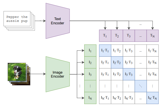
Predicting the exact words in an image-text pair was found to be wasteful in computation. Instead they adopt an approach from contrastive representation learning, predicting only if a text as a whole paired with an image makes sense:

Given a batch of $N$ (image, text) pairs, CLIP is trained to predict which of the $N \times N$ possible (image, text) pairs across a batch occurred. To do this the model needs an image and a text encoder that embed into the same space. The goal is then to maximize the cosine similarity between the image and text embeddings in the $N$ pairs, while minimizing the cosine similarity of the $N^2-N$ incorrect pairings. This is done with a symmetric cross entropy loss over all the similarity scores. Clip is trained from scratch without initializing the image encoder or the text encoder. The embeddings are then created with a linear projection to the multimodal embedding space.

Clip pre-training setup matrix of text and image embeddings.

The symmetric cross-entropy loss for clip for $N$ text-image embedding pairs $(t, i) \in (T,I)$ and temperature $t$ :

$L_{clip}(T, I) = \frac{1}{2}\big(L_{CE}(T, I) + L_{RCE}(I, T)\big)$

Pseudo code for CLIP loss:

# image_encoder - ResNet or Vision Transformer
# text_encoder - CBOW or Text Transformer
# I[n, h, w, c] - minibatch of aligned images
# T[n, l] - minibatch of aligned texts
# W_i[d_i, d_e] - learned proj of image to embed
# W_t[d_t, d_e] - learned proj of text to embed
# t - learned temperature parameter
# extract feature representations of each modality
I_f = image_encoder(I) #[n, d_i]
T_f = text_encoder(T) #[n, d_t]
# joint multimodal embedding 
# normalize embeddings to unit length for cosine similarity
I_e = l2_normalize(np.dot(I_f, W_i), axis=1) # [n, d_e]
T_e = l2_normalize(np.dot(T_f, W_t), axis=1) # [n, d_e]
# temperature scaled pairwise cosine similarities 
logits = np.dot(I_e, T_e.T) * np.exp(t) # [n, n]
# symmetric cross-entropy loss function
labels = np.arange(n) 
# diagonal is 1 and off-diagonal is zero
loss_i = cross_entropy_loss(logits, labels, axis=0)
loss_t = cross_entropy_loss(logits, labels, axis=1)
loss = (loss_i + loss_t)/2

Prompt Engineering

The model is embedding entire sentences and not just words, this allows for using prompt engineering to improve results. For example a common issue with only using single words is that they can have multiple meanings without context (maybe even with context). One example from ImageNet is construction cranes and the animal cranes that fly.

Another issue is that in pre-training the images will often be paired with entire sentences (alt-text) and not single words, this means at inference time using single words will be out of distribution as a task.

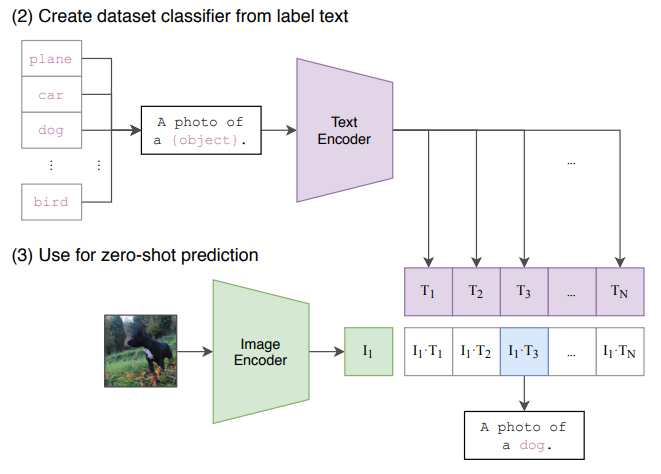
The paper uses a simple prompt template “A photo of a {label}” as a default. This default is then often adapted to each task.

How CLIP does inference with zero shot prediction.

Another option to increase performance is to ensemble over many different context prompts, which lead to an improvement of 3.5% over the default prompt.

The paper presents many results on different tasks that we will not get into here. One of the main take-aways is that CLIP features outperform the features of an ImageNet pre-trained model on a wide variety of datasets. They are also more robust to task shift compared to ImageNet models.

One interesting result was comparing CLIP to zero, one and two shot humans.

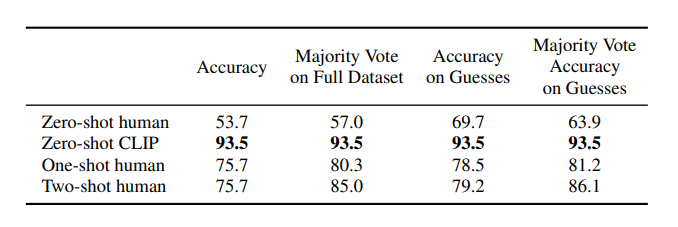
How CLIP compares to humans in zero, one and two shot regime.

Humans know what they don’t know, and can generalize much better from one example, as evidenced by the large jump in accuracy. This point is still valid for LLMs today in 2025. They can’t tell us what they don’t know and tend to hallucinate instead. One could argue that they are better these days with generalizing from few examples in few-shot prompts, but that has its limits as well as any practitioner can tell.

Sigmoid Language Image Pretraining - 2022 to 2025

These are a series of papers by (now former) Google researchers in Zurich. They build upon the ideas from CLIP, among many others, to create one of the best open source image backbones.

LiT: Zero-Shot Transfer with locked Image-Text Tuning - 2022

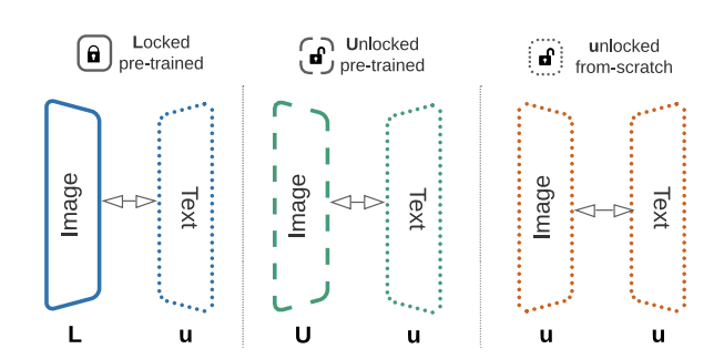
The paper presents a contrastive tuning method to align image and text models, while taking advantage of pre-trained models. Here this is called “Locked-image Tuning” (LiT). It teaches a text model to read representations from pre-trained image models for new tasks. It works for multiple vision architectures.

The main contribution from paper is a strategy they call contrastive tuning. It consists of only tuning the text tower while using a pre-trained image backbone. This is called locked-image tuning because the image tower is frozen (locked) during training.

This achieves better results than from scratch training like CLIP.

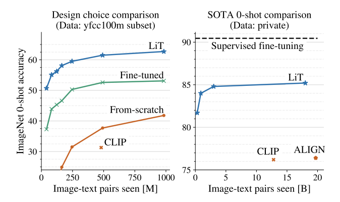
Figure 1 from paper comparing performances of previous SOTA methods.

The paper also tests multiple variants:

Initialize from pre-trained models, train text only.
Initialize from pre-trained models, train text and image.
Initialize randomly, train text and image.

The image denotes this in L (locked and pre-trained), U (unlocked and pre-trained) and u (unlocked and randomly initialized).

Figure 2 from paper showing which parts of the model can be locked or unlocked at same time.

The two models are trained with a contrastive loss as in CLIP. They ablate if it should be calculated on a per accelerator basis or computed jointly across devices. The second version consistently gives better results. This intuitively makes sense and we will see in later papers that a certain batch size is necessary for the contrastive loss to work well.

Contrastive pre-training can be viewed as learning two tasks at the same time:

1) Learning an image embedding

2) Learning a text embedding to align with image embedding space.

Contrastive pre-training works well for both of these tasks but might not be the optimal approach, hence these experiments.

Again the two options at the time were pre-training image models on a fixed set of categories like ImageNet-21k or JFT-300M, or do free-from pre-training on image-text pairs from the internet.

The first approach has cleaner data but the categories the image model learns are restricted to those in the training set. There is no guarantee that the embeddings work well outside of categories. And experience tells me that it probably won’t.

The second approach has orders of magnitude more data available (as we will see in the next papers) and tends to generalize much better, even though the labels are of weaker quality. This might not be a surprise after the LLM revolution in the past years.

Sigmoid Loss for Language Image Pre-Training - 2023

The main contribution of this paper was a new loss for contrastive pre-training. Unlike the previously seen loss which uses softmax normalization, the sigmoid loss only operates on image-text pairs and we do not need a global view of the pairwise similarities for normalization. This allows increased batch size while also improving the performance at smaller batch sizes.

The disentanglement from batch size and loss allowed for further studying of impact of the ratio of positive to negative examples in a batch. Before this was fixed at $N^2$ pairs of which $N$ were positive and $N^2-N$ were negative.

Theoretical Method

For:

$f(\cdot)$ an image model.
$g(\cdot)$ a text model.
$B = \lbrace (I_1, T_1), (I_2, T_2), \cdots \rbrace$ a mini-batch of image-text pairs.
$N = \mid B \mid$ the mini-batch size.
$x_i = \frac{f(I_i)}{\mid \mid f(I_i) \mid \mid_2}$ a normalized image embedding.
$y_i = \frac{g(T_i)}{\mid \mid g(T_i) \mid \mid_2}$ a normalized text embedding.
$t$ a scalar parametrized as $\exp(t')$ , where $t'$ is a freely learnable parameter.

The softmax loss for contrastive learning is:

$L_{softmax} = \frac{1}{2N} \sum_{i=1}^{N} \left( \log \frac{e^{t x_i y_i}}{\sum_{j=1}^{N} e^{t x_i y_j}} + \log \frac{e^{t x_i y_i}}{\sum_{j=1}^{N} e^{t x_i y_j}} \right)$

The first part in the sum is image to text softmax, the second is text to image softmax. Note, due to the asymmetry of the softmax loss, the normalization is independently performed two times: across images and across texts.

In case of the sigmoid loss, we do not require computing global normalization factors. Every image-text pair is processed independently. Turning the problem into a standard binary classification problem of all pair combinations. So for image-text pairs $(I_i, T_j)$ we have $z_{ij} = 1$ for $i=j$ and $z_{ij} = -1$ if $i \neq j$ . The loss is defined as:

$L_{sig} = - \frac{1}{N} \sum^{N}_{i=1} \sum^{N}_{j=1} \log \frac{1}{1+e^{z_{ij}(-tx_i y_j + b)}}$ .

There is a new bias term $b$ in this loss to correct for the heavy imbalance of many negatives that dominate the loss initially. The two terms are initialized as:

$t'= \log(10)$ for the temperature $t$
$b = -10$ for the bias $b$ .

This assures that the training starts close to the prior and does not require over-correction.

Question: what is the prior here?

The pseudocode implementation of this loss is:

# img_emb : image model embedding [n, dim] 
# txt_emb : text model embedding [n, dim] 
# t_prime, b : learnable temperature and bias 
# n : mini-batch size 
 
t = exp(t_prime) 
zimg = l2_normalize(img_emb) 
ztxt = l2_normalize(txt_emb) 
logits = dot(zimg, ztxt.T) * t + b 
labels = 2 * eye(n) - ones(n) # Create a matrix with 1s on the diagonal and -1 elsewhere
l = -sum(log_sigmoid(labels * logits)) / n

Practical Considerations

Contrastive learning in the form of the softmax loss typically uses data parallelism, computing the loss when data is split across $D$ devices is expensive because we need to gather all embeddings with expensive all-gather operations. And the materialization of a $N \times N$ matrix of pairwise similarities.

For the sigmoid loss a more efficient implementation exists that avoids these issues. If we assume that each device holds $b = \frac{N}{D}$ examples, then for each example we have one positive and $b-1$ negatives on the device. Then the text representations are permitted among the devices to calculate $b$ negative examples with each step. The loss is calculated on a per device basis for each local batch $b$ and summed up across devices. The process if visualized in the following image for three devices and four examples per device:

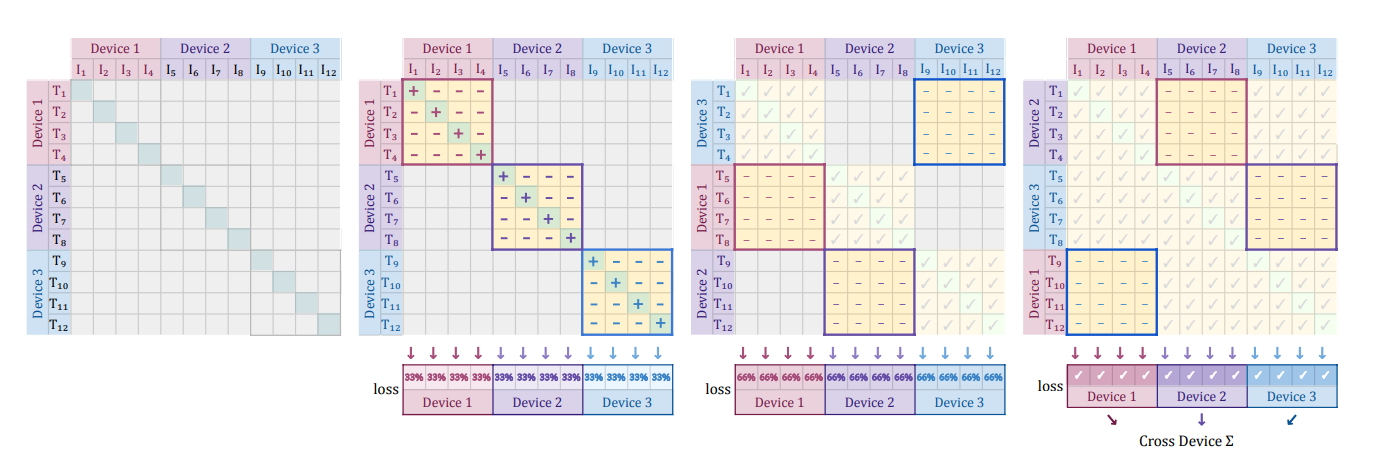
Figure 1 from paper showing how the text embeddings get propagated to calculate the complete loss.

The peak memory cost is reduced from $N^2$ to $b^2$ , and $b$ can be kept constant while scaling up accelerators. This allows much larger batch sizes than the original cross-entropy loss.

There is a lot more engineering details and considerations in the paper that I don’t want to go into too many details here:

SigLIP works better for smaller batch sizes, but at larger batch sizes like 32k softmax loss catches up. Larger batch sizes make more sense if training for longer, on ImageNet zero-shot transfer.
Increased batch size leads to increased training instability due to spikes in gradient norm, decreasing $\beta_2$ momentum helps.
Loss paradigm: softmax “pick the right class” vs. sigmoid “rate this pair”.
Sigmoid loss allows to remove negatives from the training process, the only way to not decrease performance significantly is to keep the “hard examples”. Which intuitively makes the most sense, since learning is done on these. Here by hard examples we mean examples where the model makes large mistakes.

SigLIP 2: Multilingual Vision-Language Encoders - 2025

This paper extends the original paper in multiple ways:

caption based pre-training
self-supervised losses
online data curation

which leads to better performance on dense prediction tasks. Additionally there are versions which support different resolutions and aspect ratios.

Sadly the paper is devoid of any explicit loss functions, those have to be collected from the original papers that the authors mention:

LocCa: Visual pretraining with location-aware captioners.
SILC: Improving vision language pretraining with self-distillation
TIPS: Text-image pretraining with spatial awareness

Figure 1 from paper showing which additional parts are added to the training process compared to the original SigLip.

New Training Regime

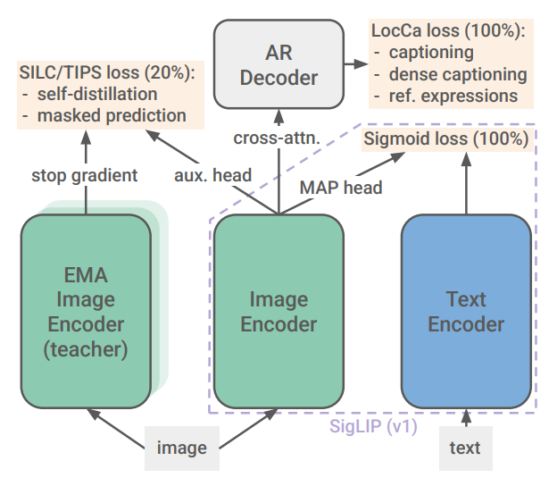
The training process builds on the original SigLIP process by adding self-distillation and masked prediction tasks. This is done in a staged approach and with multiple loss functions.

SigLIP loss

As described in the chapter above. Pairwise binary classification loss.

LocCa loss

LocCa trains for automatic referring expression prediction (bounding box prediction for specific image regions) and grounded captioning (predicting region specific captions given BBox coordinates).

Local to Global consistency loss - SLIC

The vision encoder becomes the student network which gets a partial local view of the training image, and is trained to match the teachers representation. The teacher saw the full image. The teacher is an exponential moving average of the students parameters.

Masked Prediction Objective - TIPS

50% of the embedded image patches in the student network are replaced with mask tokens. The student then has to match the features from the teacher at the masked location.

This loss is applied to per-patch features rather than the pooled image-level representations. Both the student and the teacher see the same global view of the image.

The latter two losses are only added at 80% of the training process. Additionally they are only applied to augmented images, not the original one.

Conclusion

We saw a stream of papers and interesting ideas from the CLIP research branch that show us how to train state of the art image encoders in 2025. This is done by using unsupervised or semi-supervised training methods together with large amounts of noisy data, lots of compute and some clever engineering (softmax vs sigmoid).

Final Thoughts

Some follow up questions and remarks for my future self or experts in this field:

Similarly to LLMs, we seem to run out of training data as WebLI represents the entire (high quality) internet data, what else can be done? Generate more data with GenAI and use captioning for training smaller models?
Are there any tasks that are not covered yet with the current training approaches?
Could we use videos as another data source for further advances?
A very 2025 take, can we apply RL to improve vision further? Explored to some extend already in 2023 by the Big Vision team.

References

A list of resources used to write this post, also useful for further reading:

Learning Transferable Visual Models From Natural Language Supervision - Alec Radford, Jong Wook Kim, Chris Hallacy, Aditya Ramesh, Gabriel Goh, Sandhini Agarwal, Girish Sastry, Amanda Askell, Pamela Mishkin, Jack Clark, Gretchen Krueger, Ilya Sutskever for the CLIP paper that started it all.
LiT: Zero-Shot Transfer with Locked-image text Tuning - Xiaohua Zhai, Xiao Wang, Basil Mustafa, Andreas Steiner, Daniel Keysers, Alexander Kolesnikov, Lucas Beyer for the follow up paper where only one part is tuned.
Sigmoid Loss for Language Image Pre-Training - Xiaohua Zhai, Basil Mustafa, Alexander Kolesnikov, Lucas Beyer for the SigLIP paper that introduced the simplified loss and many valuable open source models.
SigLIP 2: Multilingual Vision-Language Encoders with Improved Semantic Understanding, Localization, and Dense Features - Michael Tschannen, Alexey Gritsenko, Xiao Wang, Muhammad Ferjad Naeem, Ibrahim Alabdulmohsin, Nikhil Parthasarathy, Talfan Evans, Lucas Beyer, Ye Xia, Basil Mustafa, Olivier Hénaff, Jeremiah Harmsen, Andreas Steiner, Xiaohua Zhai for the follow up to the original SigLIP paper.
LocCa: Visual Pretraining with Location-aware Captioners - Bo Wan, Michael Tschannen, Yongqin Xian, Filip Pavetic, Ibrahim Alabdulmohsin, Xiao Wang, André Susano Pinto, Andreas Steiner, Lucas Beyer, Xiaohua Zhai for the LocCa loss used in SigLIP2.
SILC: Improving Vision Language Pretraining with Self-Distillation - Muhammad Ferjad Naeem, Yongqin Xian, Xiaohua Zhai, Lukas Hoyer, Luc Van Gool, Federico Tombari for the SLIC loss used in the SigLIP2 paper.
TIPS: Text-Image Pretraining with Spatial Awareness - Kevis-Kokitsi Maninis, Kaifeng Chen, Soham Ghosh, Arjun Karpur, Koert Chen, Ye Xia, Bingyi Cao, Daniel Salz, Guangxing Han, Jan Dlabal, Dan Gnanapragasam, Mojtaba Seyedhosseini, Howard Zhou, Andre Araujo for the TIPS loss used in the SigLIP2 paper.

Comments

I would be happy to hear about any mistakes or inconsistencies in my post. Other suggestions are of course also welcome. You can either write a comment below or find my email address on the about page.

Combining Vision and Language

On combining large vision and language models.